Modeling synapses in NESTML

Conceptually, a synapse model formalises the interaction between two (or more) neurons. In biophysical terms, they may contain some elements that are part of the postsynaptic neuron (such as the postsynaptic density) as well as the presynaptic neuron (such as the vesicle pool), or external factors such as the concentration of an extracellular diffusing factor. We will discuss in detail the spike-timing dependent plasticity (STDP) model and some of its variants.

From the modeling point of view, a synapse shares many of the same behaviours of a neuron: it has parameters and internal state variables, can communicate over input and output ports, and its dynamics and responses can be described by differential equations, kernels and as an algorithm. Typically, there is a single spiking input port and a single spiking output port.

Attention

The NEST Simulator platform target has some additional constraints, such as precluding updates on a regular time grid. See The NEST target for more details.

Key to writing the synapse model is the requirement that the event handler for the spiking input port is responsible for submitting the event to the (spiking) output port.

Note that the synaptic strength (“weight”) variable is of type real; if the type were given in more specific units, such as nS or pA, the synapse model would only be compatible with either a conductance or current-based postsynaptic neuron model.

Writing the NESTML model

The top-level element of the model is synapse, followed by a name. All other blocks appear inside of here.

synapse stdp:
    # [...]

Input and output ports

Depending on whether the plasticity rule depends only on pre-, or on both pre- and postsynaptic activity, one or two input ports are defined. Synapses always have only one (spiking) output port.

input:
    pre_spikes <- spike
    post_spikes <- spike

output: spike

Presynaptic spike event handler

It is the responsibility of the event handler for the spiking input port to submit the event to the (spiking) output port. This can be done using the predefined deliver_spike(w, d) function, which takes two parameters: a weight w and delay d.

The corresponding event handler has the general structure:

onReceive(pre_spikes):
    print("Info: processing a presynaptic spike at time t = {t}")
    # ... plasticity dynamics go here ...
    deliver_spike(w, d)

The statements in the event handler will be executed sequentially when the event occurs. The weight and delay could be defined as follows:

state:
    w real = 1

parameters:
    d ms = 1 ms

If synaptic plasticity modifies the weight of the synapse, the weight update could (but does not have to) take place before calling deliver_spike() with the updated weight.

State variables (in particular, synaptic “trace” variables as often used in plasticity models) can be updated in the event handler as follows:

state:
    tr_pre real = 0

onReceive(post_spikes):
    print("Info: processing a presynaptic spike at time t = {t}")
    tr_pre += 1

equations:
    tr_pre' = -tr_pre / tau_tr

Equivalently, the trace can be defined as a convolution between a trace kernel and the spiking input port:

equations:
    kernel tr_pre_kernel = exp(-t / tau_tr)
    inline tr_pre real = convolve(tr_pre_kernel, pre_spikes)

Postsynaptic spike event handler

Some plasticity rules are defined in terms of postsynaptic spike activity. A corresponding additional spiking input port and event handler (and convolutions) can be defined in the NESTML model:

input:
    pre_spikes <- spike  # (same as before)
    post_spikes <- spike

onReceive(post_spikes):
    print("Info: processing a postsynaptic spike at time t = {t}")
    # ... plasticity dynamics go here ...

Sharing parameters between synapses

If one or more synapse parameters are the same across a population (homogeneous), then sharing the parameter value between all synapses can save vast amounts of memory. To mark a particular parameter as homogeneous, use the @homogeneous decorator keyword. This can be done on a per-parameter basis.

By default, parameters are heterogeneous which means can be set on a per-synapse basis by the user.

For example:

parameters:
    a real = 3.14159   @homogeneous
    b real = 100.      @heterogeneous  # the default!

Third-factor plasticity

The postsynaptic trace value in the models so far is assumed to correspond to a property of the postsynaptic neuron, but it is specified in the synapse model. Some synaptic plasticity rules require access to a postsynaptic value that cannot be specified as part of the synapse model, but is a part of the (postsynaptic) neuron model.

An example would be a neuron that generates dendritic action potentials. The synapse could need access to the postsynaptic dendritic current. For more details on this example, please see the tutorial https://nestml.readthedocs.io/en/latest/tutorials/active_dendrite/nestml_active_dendrite_tutorial.html

An additional complication is that when combining models from different sources, the naming convention can be different between the neuron and synapse model.

To make the “third factor” value available in the synapse model, begin by defining an appropriate input port:

input:
    I_post_dend pA <- continuous

In the synapse, the value will be referred to as I_post_dend and can be used in equations and expressions. In this example, we will use it as a simple gating variable between 0 and 1, that can disable or enable weight updates in a graded manner:

onReceive(post_spikes):
    # potentiate synapse
    w_ real = # [...] normal STDP update rule
    w_ = (I_post_dend / pA) * w_ + (1 - I_post_dend / pA) * w   # "gating" of the weight update
    w = min(Wmax, w_)

In the neuron, no special output port is required; all state variables are accessible for the third factor rules.

NESTML needs to be invoked so that it generates code for neuron and synapse together. Additionally, specify the "post_ports" entry to connect the input port on the synapse with the right variable of the neuron (see Generating code).

In this example, the I_dend state variable of the neuron will be simply an exponentially decaying function of time, which can be set to 1 at predefined times in the simulation script. By inspecting the magnitude of the weight updates, we see that the synaptic plasticity is indeed being gated by the neuronal state variable (“third factor”) I_dend.

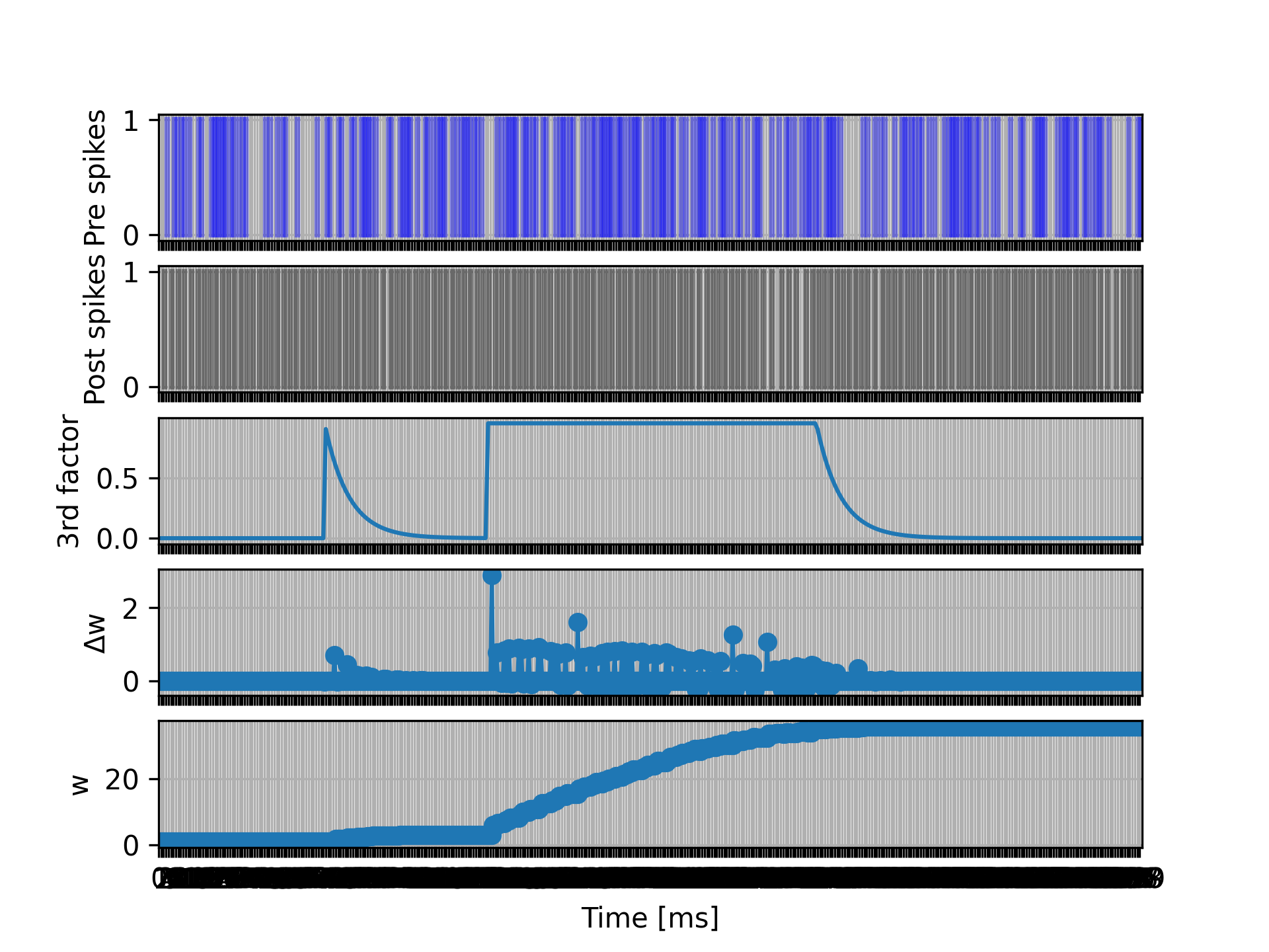
For a full example, please see the following files:

• tests/nest_tests/third_factor_stdp_synapse_test.py (produces the figure)

• models/neurons/iaf_psc_exp_dend.nestml (neuron model)

• models/synapses/third_factor_stdp_synapse.nestml (synapse model)

Examples

Spike-Timing Dependent Plasticity (STDP)

Experiments have shown that synaptic strength changes as a function of the precise spike timing of the presynaptic and postsynaptic neurons. If the pre neuron fires an action potential strictly before the post neuron, the synapse connecting them will be strengthened (“facilitated”). If the pre neuron fires after the post neuron, the synapse will be weakened (“depressed”). The depression and facilitation effects become stronger when the spikes occur closer together in time. This is illustrated by empirical results (open circles), fitted by exponential curves (solid lines).

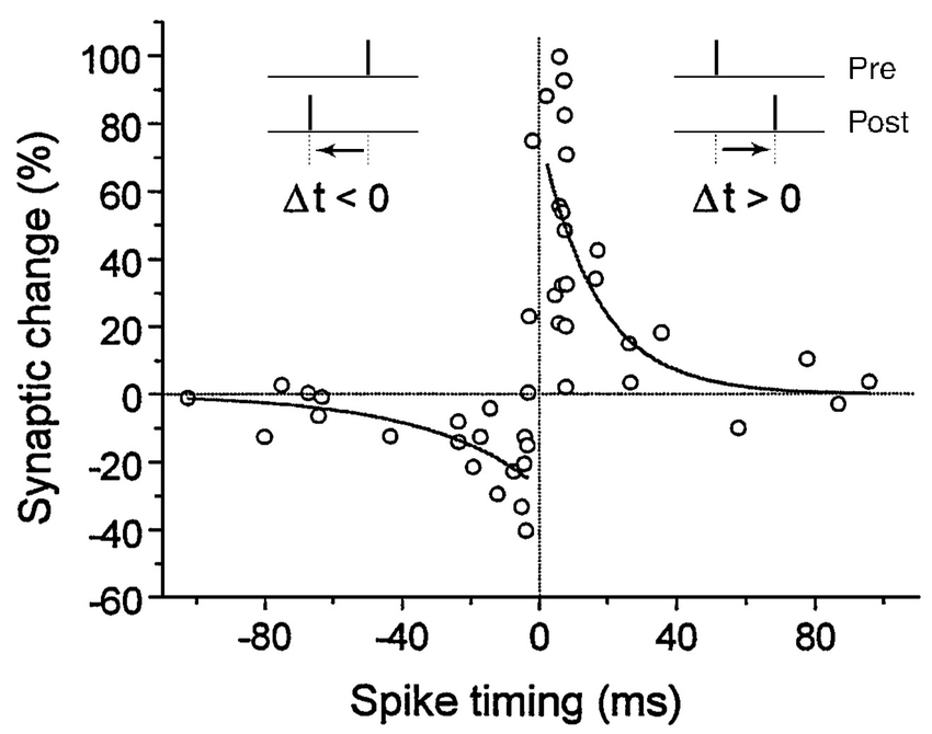
Figure 1 Asymmetric STDP learning window. Spike-timing window of STDP for the induction of synaptic potentiation and depression characterized in hippocampal cultures. Data points from Bi and Poo (1998), represent the relative change in the amplitude of EPSC after repetitive correlated activity of pre-post spike pairs. The potentiation window (right of the vertical axis) and depression window (left of the vertical axis) are fitted by an exponential function $A^pmexp(−|Delta t|/tau^pm)$, with parameters $A^+ = 0.86$, $A^- = -0.25$, $tau^+ = 19 text{ms}$, and $tau^- = 34 text{ms}$. Adopted from Bi and Wang (2002).

We will define the theoretical model following [3].

A pair of spikes in the input and the output cell, at times \(t_i\) and \(t_j\) respectively, induces a change \(\Delta w\) in the weight \(w\):

\[\Delta^\pm w = \pm \lambda \cdot f_\pm(w) \cdot K(|t_o - t_i|)\]

The weight is increased by \(\Delta^+ w\) when \(t_o>t_i\) and decreased by \(\Delta^- w\) when \(t_i>t_o\). The temporal dependence of the update is defined by the filter kernel \(K\) which is taken to be \(K(t) = \exp(-t/\tau)\). The coefficient \(\lambda\in\mathbb{R}\) sets the magnitude of the update. The functions \(f_\pm(w)\) determine the relative magnitude of the changes in the positive and negative direction. These are here taken as

\[\begin{split}\begin{align} f_+(w) &= (1 - w)^{\mu_+}\\ f_-(w) &= \alpha w^{\mu_-} \end{align}\end{split}\]

with the parameter \(\alpha\in\mathbb{R}, \alpha>0\) allowing to set an asymmetry between increasing and decreasing the synaptic efficacy, and \(\mu_\pm\in\{0,1\}\) allowing to choose between four different kinds of STDP (for references, see https://nest-simulator.readthedocs.io/en/nest-2.20.1/models/stdp.html?highlight=stdp#_CPPv4I0EN4nest14STDPConnectionE).

To implement the kernel, we use two extra state variables, one presynaptic so-called trace value and another postsynaptic trace value. These could correspond to calcium concentration in biology, maintaing a history of recent neuron spiking activity. They are incremented by 1 whenever a spike is generated, and decay back to zero exponentially. Mathematically, this can be formulated as a convolution between the exponentially decaying kernel and the emitted spike train:

\[\text{tr_pre} = K \ast \sum_i \delta_{pre,i}\]

and

\[\text{tr_post} = K \ast \sum_i \delta_{post,i}\]

These are implemented in the NESTML model as follows:

equations:
    # all-to-all trace of presynaptic neuron
    kernel tr_pre_kernel = exp(-t / tau_tr_pre)
    inline tr_pre real = convolve(tr_pre_kernel, pre_spikes)

    # all-to-all trace of postsynaptic neuron
    kernel tr_post_kernel = exp(-t / tau_tr_post)
    inline tr_post real = convolve(tr_post_kernel, post_spikes)

with time constants defined as parameters:

parameters:
    tau_tr_pre ms = 20 ms
    tau_tr_post ms = 20 ms

With the traces in place, the weight updates can then be expressed closely following the mathematical definitions. Begin by defining the weight state variable and its initial value:

state:
    w real = 1.

Our update rule for facilitation is:

\[\Delta^+ w = \lambda \cdot (1 - w)^{\mu_+} \cdot \text{tr_pre}\]

In NESTML, this expression can be entered almost verbatim. Note that the only difference is that scaling with an absolute maximum weight Wmax was added:

onReceive(post_spikes):
    # potentiate synapse
    w_ real = Wmax * ( w / Wmax  + (lambda * ( 1. - ( w / Wmax ) )**mu_plus * tr_pre ))
    w = min(Wmax, w_)

Our update rule for depression is:

\[\Delta^- w = -\alpha \cdot \lambda \cdot w^{\mu_-} \cdot \text{tr_post}\]

onReceive(pre_spikes):
    # depress synapse
    w_ real = Wmax * ( w / Wmax  - ( alpha * lambda * ( w / Wmax )**mu_minus * tr_post ))
    w = max(Wmin, w_)

    # deliver spike to postsynaptic partner
    deliver_spike(w, d)

Finally, all remaining parameters are defined:

parameters:
    lambda real = .01
    alpha real = 1.
    mu_plus real = 1.
    mu_minus real = 1.
    Wmax real = 100.
    Wmin real = 0.

The NESTML STDP synapse integration test (tests/nest_tests/stdp_window_test.py) runs the model for a variety of pre/post spike timings, and measures the weight change numerically. We can use this to verify that our model approximates the correct STDP window. Note that the dendritic delay in this example has been set to 10 ms, to make its effect on the STDP window more clear: it is not centered around zero, but shifted to the left by the dendritic delay.

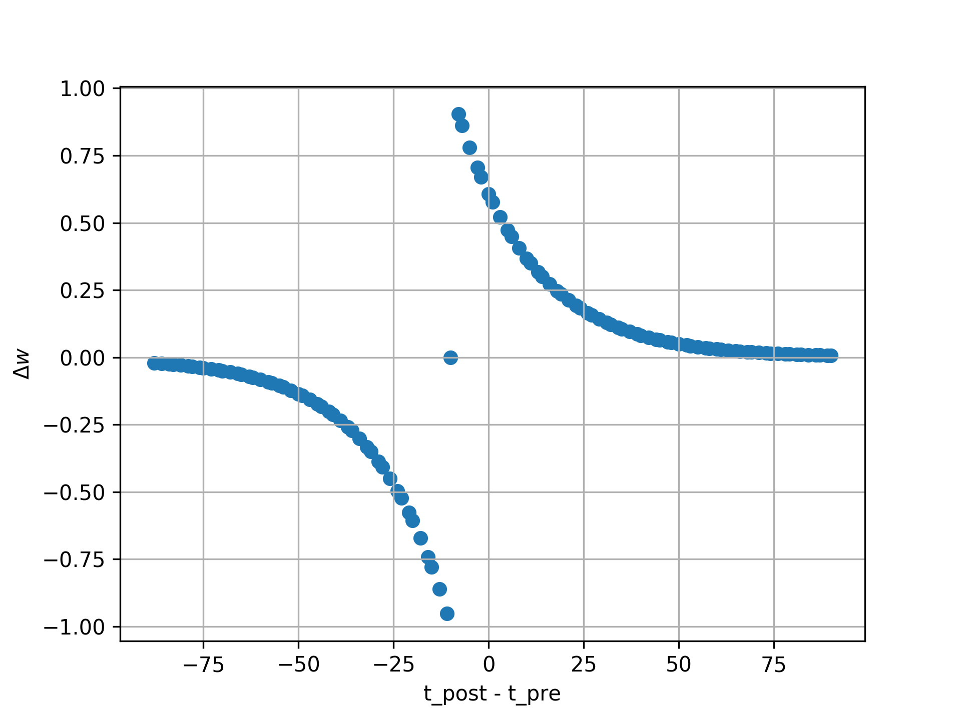
Figure 2 STDP window, obtained from numerical simulation, for purely additive STDP (mu_minus = mu_plus = 0) and a dendritic delay of 10 ms.

STDP synapse with nearest-neighbour spike pairing

This synapse model extends the STDP model by restrictions on interactions between pre- and post spikes.

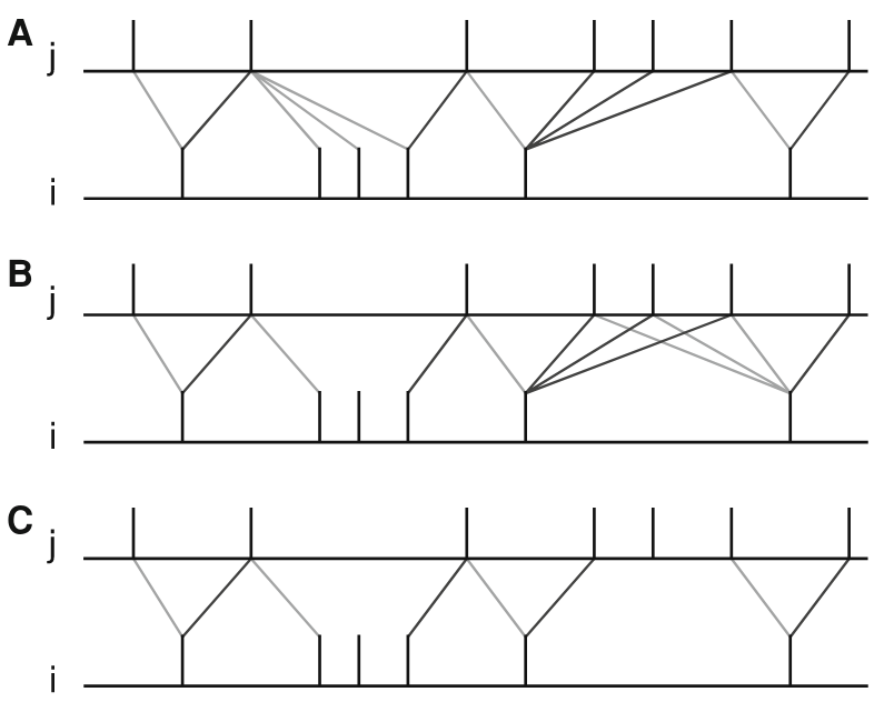
Figure 3 Figure 7 from Morrison, Diesmann and Gerstner [1]. Original caption: “Examples of nearest neighbor spike pairing schemes for a pre-synaptic neuron j and a postsynaptic neuron i. In each case, the dark gray indicate which pairings contribute toward depression of a synapse, and light gray indicate which pairings contribute toward potentiation. (a) Symmetric interpretation: each presynaptic spike is paired with the last postsynaptic spike, and each postsynaptic spike is paired with the last presynaptic spike (Morrison et al. 2007). (b) Presynaptic centered interpretation: each presynaptic spike is paired with the last postsynaptic spike and the next postsynaptic spike (Izhikevich and Desai 2003; Burkitt et al. 2004: Model II). (c) Reduced symmetric interpretation: as in (b) but only for immediate pairings (Burkitt et al. 2004: Model IV, also implemented in hardware by Schemmel et al. 2006)”

Nearest-neighbour symmetric

This variant corresponds to panel 7A in [1]: each presynaptic spike is paired with the last postsynaptic spike, and each postsynaptic spike is paired with the last presynaptic spike.

To implement this rule, the pre- and postsynaptic traces are reset to 1 instead of incremented by 1. To implement this in the model, we define the traces are state variables and ODEs, instead of convolutions:

state:
    tr_pre real = 0.
    tr_post real = 0.

equations:
    tr_pre' = -tr_pre / tau_tr_pre
    tr_post' = -tr_post / tau_tr_post

Resetting to 1 can then be done by assignment in the pre- and post-event handler blocks:

onReceive(pre_spikes):
    tr_pre = 1
    [...]

onReceive(post_spikes):
    tr_post = 1
    [...]

The rest of the model is equivalent to the normal (all-to-all spike pairing) STDP.

The full model can be downloaded here: stdp_nn_symm.nestml.

Presynaptic centered

This variant corresponds to panel 7B in [1]: each presynaptic spike is paired with the last postsynaptic spike and the next postsynaptic spike.

To implement this rule, the postsynaptic trace is reset to 1 upon a spike, whereas the presynaptic trace is incremented by 1. Additionally, when a postsynaptic spike occurs, the presynaptic trace is reset to zero, thus “forgetting” presynaptic spike history.

onReceive(post_spikes):
    tr_post = 1
    w = ...  # facilitation step (omitted)
    tr_pre = 0

onReceive(pre_spikes):
    tr_pre += 1
    w = ...  # depression step (omitted)
    deliver_spike(w, d)

The remainder of the model is the same as the all-to-all STDP synapse.

The full model can be downloaded here: stdp_nn_pre_centered.nestml.

Restricted symmetric

This variant corresponds to panel 7C in [1]: like the Nearest-neighbour symmetric rule, but only for immediate pairings.

To implement this rule, depression and facilitation are gated through a boolean, pre_handled, which ensures that each postsynaptic spike can only pair with a single presynaptic spike.

initial_values:
    # [...]
    pre_handled boolean = True

onReceive(pre_spikes):
    # [...]

    # depress synapse
    if pre_handled:
        w = ...  # depression step (omitted)
    # [...]

onReceive(post_spikes):
    # [...]

    if not pre_handled:
        w = ...  # potentiation step (omitted)
        pre_handled = True

    # [...]

The remainder of the model is the same as the Presynaptic centered variant.

The full model can be downloaded here: stdp_nn_restr_symm.nestml.

Triplet-rule STDP synapse

Traditional STDP models express the weight change as a function of pairs of pre- and postsynaptic spikes, but these fall short in accounting for the frequency dependence of weight changes. To improve the fit between model and empirical data, [4] propose a “triplet” rule, which considers sets of three spikes, that is, two pre and one post, or one pre and two post.

Figure 4 Figure 1 from [4].

Two traces, with different time constants, are defined for both pre- and postsynaptic partners. The temporal evolution of the traces is illustrated in panels B and C: for the all-to-all variant of the rule, each trace is incremented by 1 upon a spike (panel B), whereas for the nearest-neighbour variant, each trace is reset to 1 upon a spike (panel C). The weight updates are then computed as a function of the trace values and four coefficients: a depression pair term \(A_2^-\) and triplet term \(A_3^-\), and a facilitation pair term \(A_2^+\) and triplet term \(A_3^+\). A presynaptic spike after a postsynaptic one induces depression, if the temporal difference is not much larger than \(\tau_-\) (pair term, \(A_2^−\)). The presence of a previous presynaptic spike gives an additional contribution (2-pre-1-post triplet term, \(A_3^−\)) if the interval between the two presynaptic spikes is not much larger than \(\tau_x\). Similarly, the triplet term for potentiation depends on one presynaptic spike but two postsynaptic spikes. The presynaptic spike must occur before the second postsynaptic one with a temporal difference not much larger than \(\tau_+\).

parameters:
    tau_plus ms = 16.8 ms   # time constant for tr_r1
    tau_x ms = 101 ms       # time constant for tr_r2
    tau_minus ms = 33.7 ms  # time constant for tr_o1
    tau_y ms = 125 ms       # time constant for tr_o2

equations:
    kernel tr_r1_kernel = exp(-t / tau_plus)
    inline tr_r1 real = convolve(tr_r1_kernel, pre_spikes)

    kernel tr_r2_kernel = exp(-t / tau_x)
    inline tr_r2 real = convolve(tr_r2_kernel, pre_spikes)

    kernel tr_o1_kernel = exp(-t / tau_minus)
    inline tr_o1 real = convolve(tr_o1_kernel, post_spikes)

    kernel tr_o2_kernel = exp(-t / tau_y)
    inline tr_o2 real = convolve(tr_o2_kernel, post_spikes)

The weight update rules can then be expressed in terms of the traces and parameters, directly following the formulation in the paper (eqs. 3 and 4, [4]):

parameters:
    A2_plus real = 7.5e-10
    A3_plus real = 9.3e-3
    A2_minus real = 7e-3
    A3_minus real = 2.3e-4

    Wmax real = 100.
    Wmin real = 0.

onReceive(post_spikes):
    # potentiate synapse
    w_ real = w + tr_r1 * ( A2_plus + A3_plus * tr_o2 )
    w = min(Wmax, w_)

onReceive(pre_spikes):
    # depress synapse
    w_ real = w  -  tr_o1 * ( A2_minus + A3_minus * tr_r2 )
    w = max(Wmin, w_)

    # deliver spike to postsynaptic partner
    deliver_spike(w, d)

Generating code

Co-generation of neuron and synapse

Most plasticity models, including all of the STDP variants discussed above, depend on the storage and maintenance of “trace” values, that record the history of pre- and postsynaptic spiking activity. The trace dynamics and parameters are part of the synaptic plasticity rule that is being modeled, so logically belong in the NESTML synapse model. However, if each synapse maintains pre- and post traces for its connected partners, and considering that a single neuron may have on the order of thousands of synapses connected to it, these traces would be stored and computed redundantly. Instead of keeping them as part of the synaptic state during simulation, they more logically belong to the neuronal state.

To prevent this redundancy, a fully automated dependency analysis is run during code generation, that identifies those variables that depend exclusively on postsynaptic spikes, and moves them into the postsynaptic neuron model. For this to work, the postsynaptic neuron model used needs to be known at the time of synaptic code generation. Thus, we need to generate code “in tandem” now for connected neuron and synapse models, hence the name “co-generation”.

To indicate which neurons will be connected to by which synapses during simulation, a list of such (neuron, synapse) pairs is passed to the code generator. This list is encoded as a JSON file. For example, if we want to use the “stdp” synapse model, connected to an “iaf_psc_exp” neuron, we would write the following:

{
  "neuron_synapse_pairs": [["iaf_psc_exp", "stdp"]]
}

This file can then be passed to NESTML when generating code on the command line. If the JSON file is named nest_code_generator_opts_triplet.json:

nestml --input_path my_models/ --codegen_opts=nest_code_generator_opts_triplet.json

Further integration with NEST Simulator is planned, to achieve a just-in-time compilation/build workflow. This would automatically generate a list of these pairs and automatically generate the requisite JSON file.

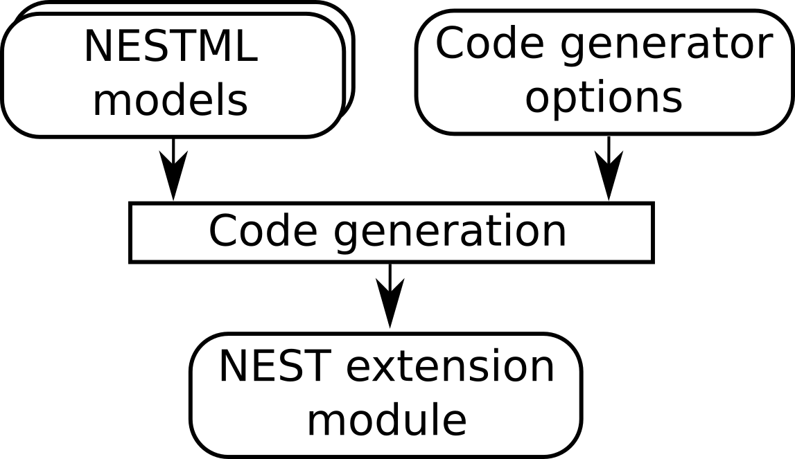
Figure 5 Code generator options instruct the target platform code generator (in this case, NEST) how to process the models.

The NEST target

Event-based updating

NEST target synapses are not allowed to have any time-based internal dynamics (ODEs). This is due to the fact that synapses are, unlike nodes, not updated on a regular time grid.

The synapse is allowed to contain an update block. Statements in the update block are executed whenever the internal state of the synapse is updated from one timepoint to the next; these updates are typically triggered by incoming spikes. The NESTML resolution() function will return the time that has elapsed since the last event was handled.

Dendritic delay

In NEST, all synapses are expected to specify a nonzero dendritic delay, that is, the delay between arrival of a spike at the dendritic spine and the time at which its effects are felt at the soma (or conversely, the delay between a somatic action potential and the arrival at the dendritic spine due to dendritic backpropagation). To indicate that a given parameter is specifying this NEST-specific delay value, use an annotation:

parameters:
    dend_delay ms = 1 ms     @nest::delay

Generating code

When NESTML is invoked to generate code for plastic synapses, the code generator needs to know which neuron model the synapses will be connected to, so that it can generate fast C++ code for the neuron and the synapse that is mutually dependent at runtime. These pairs can be specified as a list of two-element dictionaries of the form :python:`{"neuron": "neuron_model_name", "synapse": "synapse_model_name"}`, for example:

generate_target(...,
                codegen_opts={...,
                              "neuron_synapse_pairs": [{"neuron": "iaf_psc_exp_dend",
                                                        "synapse": "third_factor_stdp"}]})

Additionally, if the synapse requires it, specify the "post_ports" entry to connect the input port on the synapse with the right variable of the postsynaptic neuron:

generate_target(...,
                codegen_opts={...,
                              "neuron_synapse_pairs": [{"neuron": "iaf_psc_exp_dend",
                                                        "synapse": "third_factor_stdp",
                                                        "post_ports": ["post_spikes",
                                                                       ["I_post_dend", "I_dend"]]}]})

This specifies that the neuron iaf_psc_exp_dend has to be generated paired with the synapse third_factor_stdp, and that the input ports post_spikes and I_post_dend in the synapse are to be connected to the postsynaptic partner. For the I_post_dend input port, the corresponding variable in the (postsynaptic) neuron is called I_dend.

Simulation of volume-transmitted neuromodulation in NEST can be done using “volume transmitter” devices [5]. These are event-based and should correspond to a “spike” type input port in NESTML. The code generator options keyword “vt_ports” can be used here.

generate_target(...,
                codegen_opts={...,
                              "neuron_synapse_pairs": [{"neuron": "iaf_psc_exp_dend",
                                                        "synapse": "third_factor_stdp",
                                                         "vt_ports": ["dopa_spikes"]}]})

Implementation notes

Note that access_counter now has an extra multiplicative factor equal to the number of trace values that exist, so that spikes are removed from the history only after they have been read out for the sake of computing each trace.

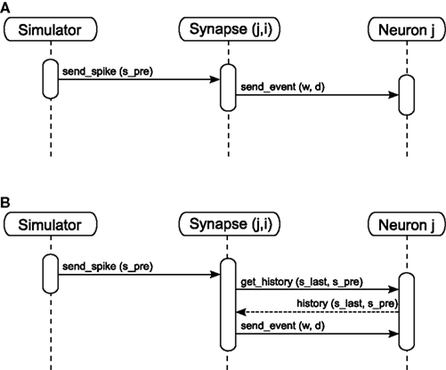
Figure 6 Potjans et al. 2010

Random numbers

In case random numbers are needed inside the synapse, the random number generator belonging to the postsynaptic target is used.

References

[1] (1,2,3,4)

Morrison A., Diesmann M., and Gerstner W. (2008) Phenomenological models of synaptic plasticity based on spike timing, Biol. Cybern. 98, 459–478

[2]

Front. Comput. Neurosci., 23 November 2010 | https://doi.org/10.3389/fncom.2010.00141 Enabling functional neural circuit simulations with distributed computing of neuromodulated plasticity, Wiebke Potjans, Abigail Morrison and Markus Diesmann

[3]

Rubin, Lee and Sompolinsky. Equilibrium Properties of Temporally Asymmetric Hebbian Plasticity. Physical Review Letters, 8 Jan 2001, Vol 86, No 2

[4] (1,2,3)

Pfister JP, Gerstner W (2006). Triplets of spikes in a model of spike timing-dependent plasticity. The Journal of Neuroscience 26(38):9673-9682. DOI: https://doi.org/10.1523/JNEUROSCI.1425-06.2006

[5]

Potjans W, Morrison A and Diesmann M (2010) Enabling functional neural circuit simulations with distributed computing of neuromodulated plasticity. Front. Comput. Neurosci. 4:141. doi: 10.3389/fncom.2010.00141