NESTML language concepts

Structure and indentation

NESTML uses Python-like indentation to group statements into blocks. Leading whitespace (spaces or tabs) determine the level of indentation. There is no prescribed indentation depth, as long as each individual block maintains a consistent level. To indicate the end of a block, the indentation of subsequent statements (after the block) must again be on the same indentation level as the code before the block has started. The different kinds of blocks can be Functions, Control structures, or any of the blocks in Block types. As an example, the following model is written with our recommended indentation level of 4 spaces:

model test:
    state:
        foo integer = 42
        bar s = 0 s

    update:
        if foo > 42:
            bar += 1 ms
        else:
            bar -= 1 ms

Similar to Python, a single line can be split into multiple lines by using a backslash (\). For example, the expression in the update block of the model below is split into multiple lines using this technique.

model test:
    state:
        tau ms = 42 ms
        foo s = 0 s

    update:
        foo = tau > 0 \
            ? foo + 1 \
            : foo - 1

Data types and physical units

Data types define types of variables as well as parameters and return values of functions. NESTML provides the following primitive types and physical data types:

Primitive data types

• real corresponds to the double data type in C++. Example literals are: 42.0, -0.42, .44

• integer corresponds to the long data type in C++. Example literals are: 42, -7

• boolean corresponds to the bool data type in C++. Its only literals are true and false

• string corresponds to the std::string data type in C++. Example literals are: "Bob", "", "Hello World!"

• void corresponds to the void data type in C++. No literals are possible and this can only be used in the declaration of a function without a return value.

Physical units

A physical unit in NESTML can be either a simple physical unit or a complex physical unit. A simple physical unit is composed of an optional magnitude prefix and the name of the unit.

The following table lists seven base units, which can be used to specify any physical unit. This idea is based on the SI units.

Quantity	Unit Name	NESTML/SI unit
length	meter	m
mass	kilogram	kg
time	second	s
electric current	ampere	A
temperature	kelvin	K
amount of substance	mole	mol
luminous intensity	candela	cd

Any other physical unit can be expressed as a combination of these seven units. These other units are called derived units. NESTML provides a concept for the derivation of new physical units, i.e., by combining simple units (consisting of a prefix and an SI unit), the user is able to create arbitrary physical units.

Units can have at most one of the following magnitude prefixes:

Factor	SI Name	NESTML prefix	Factor	SI Name	NESTML prefix
10^-1	deci	d	10^1	deca	da
10^-2	centi	c	10^2	hecto	h
10^-3	milli	m	10^3	kilo	k
10^-6	micro	u	10^6	mega	M
10^-9	nano	n	10^9	giga	G
10^-12	pico	p	10^12	tera	T
10^-15	femto	f	10^15	peta	P
10^-18	atto	a	10^18	exa	E
10^-21	zepto	z	10^21	zetta	Z
10^-24	yocto	y	10^24	yotta	Y

Simple physical units can be combined to complex units. For this, the operators , * (multiplication), / (division), ** (power) and () (parenthesis) can be used. An example could be

mV*mV*nS**2/(mS*pA)

Units of the form <unit> ** -1 can also be expressed as 1/<unit>. For example

(ms*mV)**-1

is equivalent to

1/(ms*mV)

NESTML also supports the usage of named derived-units such as Newton, Henry or lux:

Name	Symbol	Quantity	In other SI units	In base SI units
radian	rad	angle		m⋅m-1
steradian	sr	solid angle		m2⋅m−2
Hertz	Hz	frequency		s−1
Newton	N	force, weight		kg⋅m⋅s−2
Pascal	Pa	pressure, stress	N/m2	kg⋅m−1⋅s−2
Joule	J	energy, work, heat	N⋅m=Pa⋅m3	kg⋅m2⋅s−2
Watt	W	power, radiant flux	J/s	kg⋅m2⋅s−3
Coulomb	C	electric charge or quantity of electricity		s⋅A
Volt	V	voltage (electrical potential), emf	W/A	kg⋅m2⋅s−3⋅ A−1
Farad	F	capacitance	C/V	kg−1⋅ m−2⋅ s4⋅ A2
Ohm	Ω	resistance, impedance, reactance	V/A	kg⋅(m2) ⋅ (s−3) ⋅(A−2)
Siemens	S	electrical conductance	Ω−1	(kg−1) ⋅(m−2) ⋅(s3) ⋅ A2
Weber	Wb	magnetic flux	V⋅s	kg⋅(m2) ⋅(s−2) ⋅(A−1)
Tesla	T	magnetic flux density	Wb/m2	kg⋅(s−2) ⋅(A−1)
Henry	H	inductance	Wb/A	kg⋅(m2) ⋅(s−2) ⋅(A−2)
lumen	lm	luminous flux	cd⋅sr	cd
lux	lx	illuminance	lm/m2	m−2⋅ cd
Becquerel	Bq	radioactivity (decays per unit time)		s−1
Gray	Gy	absorbed dose (of ionizing radiation)	J/kg	(m2)⋅(s−2)
Sievert	Sv	equivalent dose (of ionizing radiation)	J/kg	(m2)⋅ (s−2)
katal	kat	catalytic activity		mol⋅(s−1)

Here, except for Ohm, the symbol of the unit has to be used in the model, e.g.:

x = 10 N * 22 Ohm / 0.5 V

Type and unit checks

NESTML checks type correctness of all expressions. This also applies to assignments, declarations with an initialization and function calls. NESTML supports conversion of integers to reals. A conversion between unit-typed and real-typed variables is also possible. However, these conversions are reported as warnings. Finally, there is no conversion between numeric types and boolean or string types.

Basic elements of the embedded programming language

The basic elements of the language are declarations, assignments, function calls and return statements.

Declarations

Declarations are composed of a non-empty list of comma separated names. A valid name starts with a letter, an underscore or the dollar character. Furthermore, it can contain an arbitrary number of letters, numbers, underscores and dollar characters. Formally, a valid name satisfies the following regular expression:

( 'a'..'z' | 'A'..'Z' | '_' | '$' )( 'a'..'z' | 'A'..'Z' | '_' | '0'..'9' | '$' )*

Names of functions and input ports must also satisfy this pattern. The type of the declaration can be any of the valid NESTML types. The type of the initialization expression must be compatible with the type of the declaration.

<list_of_comma_separated_names> <type> (= initialization_expression)?

a, b, c real = -0.42
d integer = 1
n integer # default value is 0
e string = "foo"
f mV = -2e12 mV

It is legal to define a variable (or kernel, or parameter) with the same name as a physical unit, but this could lead to confusion. For example, defining a variable with name b creates an ambiguity with the physical unit b, a unit of surface area. In these cases, a warning is issued when the model is processed. The variable (or kernel, and parameter) definitions will then take precedence when resolving symbols: all occurrences of the symbol in the model will be resolved to the variable rather than the unit.

For example, the following model will result in one warning and one error:

model test:
    state:
        ms mA = 42 mA   # redefine "ms" (from milliseconds unit to variable name)
        foo s = 0 s     # foo has units of time (seconds)

    update:
        ms = 1 mA    # WARNING: Variable 'ms' has the same name as a physical unit!
        foo = 42 ms  # ERROR: Actual type different from expected. Expected: 's', got: 'mA'!

Documentation string

Each model may be documented by a block of text in reStructuredText format. Following PEP 257 “Docstring Conventions”, this block should be enclosed in triple double quotes (""" ... """) and appear directly before the definition of the neuron. For example:

"""
my_custom_neuron: My customized version of a Hodgkin-Huxley model
#################################################################

Description
+++++++++++

Long description follows here. We can typeset LaTeX math:

.. math::

   E = mc^2

"""
model my_custom_neuron:
    # [...]

This documentation block is rendered as HTML on the models library.

Comments in the model

When the character # appears as the first character on a line (ignoring whitespace), the remainder of that line is allowed to contain any comment string. Comments are not interpreted as part of the model specification, but when a comment is placed in a strategic location, it will be printed into the generated NEST code.

Example of single or multi-line comments:

var1 real # single line comment

# This is
#  a comment
#   over several lines.

To enable NESTML to recognize which element a comment belongs to, the following approach has to be used: there should be no white line separating the comment and its target and the comment should be placed before the target line or on the same line as the target. For example:

# I am a comment of the membrane potential
V_m mV = -55 mV # I am a comment of the membrane potential

# I am not a comment of the membrane potential. A white line separates us.

If a comment shall be attached to an element, no white lines are allowed.

# I am not a comment of the membrane potential.

# I am a comment of the membrane potential.
V_m mV = -55 mV # I am a comment of the membrane potential

Whitelines are therefore used to separate comment targets:

# I am a comment of the membrane potential.
V_m mV = -55 mV

# I am a comment of the resting potential.
V_rest mV = -60 mV

Assignments

NESTML supports simple or compound assignments. The left-hand side of the assignment is always a variable. The right-hand side can be an arbitrary expression of a type which is compatible with the left-hand side.

Examples for valid assignments for a numeric variable n are

• simple assignment: n = 10

• compound sum: n += 10 which corresponds to n = n + 10

• compound difference: n -= 10 which corresponds to n = n - 10

• compound product: n *= 10 which corresponds to n = n * 10

• compound quotient: n /= 10 which corresponds to n = n / 10

Vectors

Variables can be declared as vectors to store an array of values. They can be declared in the parameters, state, and internals blocks. See Block types for more information on different types of blocks available in NESTML.

The declaration of a vector variable consists of the name of the variable followed by the size of the vector enclosed in [ and ]. The vector must be initialized with a default value and all the values in the vector will be initialized to the specified initial value. For example,

parameters:
    g_ex [20] mV = 10mV

Here, g_ex is a vector of size 20 and all the elements of the vector are initialized to 10mV. Note that the vector index always starts from 0. Size of the vector can be a positive integer or an integer variable previously declared in either parameters or internals block. For example, an integer variable named ten declared in the parameters block can be used to specify the size of the vector variable g_ex as:

state:
    g_ex [ten] mV = 10mV
    x [12] real = 0.

parameters:
    ten integer = 10

If the size of a vector is a variable (as ten in the above example), the vector will be resized if the value of size variable changes during the simulation. On the other hand, the vector cannot be resized if the size is a fixed integer value. Vector variables can be used in expressions as an array with an index. For example,

state:
    g_ex [ten] mV = 10mV
    x[15] real = 0.

parameters:
    ten integer = 10

update:
    integer j = 0
    g_ex[2] = -55. mV
    x[j] = g_ex[2]
    j += 1

Functions

Functions can be used to write repeatedly used code blocks only once. They consist of the function name, the list of parameters and an optional return type, if the function returns a value to the caller.

function <name>(<list_of_arguments>) <return_type>?:
    <statements>

e.g.:

function divide(a real, b real) real:
    return a/b

To use a function, it has to be called. A function call is composed of the function name and the list of required parameters. The returned value (if any) can be directly assigned to a variable of the corresponding type.

<function_name>(<list_of_arguments>)

e.g.

x = max(a*2, b/2)

Predefined functions

The following functions are predefined in NESTML and can be used out of the box. No user-defined functions can have the same name.

Name	Parameters	Description
min	x, y	Returns the minimum of x and y. Both parameters should be of the same type. The return type is equal to the type of the parameters.
max	x, y	Returns the maximum of x and y. Both parameters should be of the same type. The return type is equal to the type of the parameters.
abs	x	Returns the absolute value of x. The return type is equal to the type of x.
clip	x, y, z	Returns x if it is in [y, z], y if x < y and z if x > z. All parameter types should be the same and equal to the return type.
exp	x	Returns the exponential of x. The type of x and the return type are Real.
log10	x	Returns the base 10 logarithm of x. The type of x and the return type are Real.
ln	x	Returns the base \(e\) logarithm of x. The type of x and the return type are Real.
expm1	x	Returns the exponential of x minus 1. The type of x and the return type are Real.
sinh	x	Returns the hyperbolic sine of x. The type of x and the return type are Real.
cosh	x	Returns the hyperbolic cosine of x. The type of x and the return type are Real.
tanh	x	Returns the hyperbolic tangent of x. The type of x and the return type are Real.
erf	x	Returns the error function of x. The type of x and the return type are Real.
erfc	x	Returns the complementary error function of x. The type of x and the return type are Real.
ceil	x	Returns the ceil of x. The type of x and the return type are Real.
floor	x	Returns the floor of x. The type of x and the return type are Real.
round	x	Returns the rounded value of x. The type of x and the return type are Real.
random_normal	mean, std	Returns a sample from a normal (Gaussian) distribution with parameters “mean” and “standard deviation”
random_poisson	rate	Returns a sample from a Poissonian distribution with rate parameter (expected value) “rate”.
random_uniform	offset, scale	Returns a sample from a uniform distribution in the interval [offset, offset + scale)
delta	t	A Dirac delta impulse function at time t.
convolve	f, g	The convolution of kernel f with spike input port g.
info	s	Log the string s with logging level “info”.
warning	s	Log the string s with logging level “warning”.
print	s	Print the string s to stdout (no line break at the end). See Print function for more information.
println	s	Print the string s to stdout (with a line break at the end). See Print function for more information.
integrate_odes		This function can be used to integrate all stated differential equations of the equations block.
emit_spike		Calling this function in the update block results in firing a spike to all target neurons and devices time stamped with the current simulation time.
steps	t	Convert a time into a number of simulation steps. See the section Handling of time for more information.
resolution		Returns the current resolution of the simulation in ms. See the section Handling of time for more information.

Predefined variables and constants

The following variables and constants are predefined in NESTML and can be used out of the box. No user-defined variables can have the same name.

Name	Description
t	The current simulation time (read only)
e	Euler’s constant (2.718…)
inf	Floating point infinity

Return statement

The return keyword can only be used inside of the function block. Depending on the return type (if any), it is followed by an expression of that type.

return (<expression>)?

e.g.

if a > b:
    return a
else:
    return b

Print function

The print and println functions print a string to the standard output, with println printing a line break at the end. They can be used in the update block. See Block types for more information on the update block.

Example:

update:
    print("Hello World")
    ...
    println("Another statement")

Variables defined in the model can be printed by enclosing them in { and }. For example, variables V_m and V_thr used in the model can be printed as:

update:
    ...
    print("A spike event with membrane voltage: {V_m}")
    ...
    println("Membrane voltage {V_m} is less than the threshold {V_thr}")

Control structures

To control the flow of execution, NESTML supports loops and conditionals.

Loops

The start of the while loop is composed of the keyword while followed by a boolean condition and a colon. It executes the statements inside the block as long as the given boolean expression evaluates to true.

while <boolean_expression>:
    <statements>

e.g.:

x integer = 0
while x <= 10:
    y = max(3, x)

The for loop starts with the keyword for followed by the name of a previously defined variable of type integer or real. The fist variant uses an integer stepper variable which iterates over the half-open interval [lower_bound, upper_bound) in steps of 1.

for <existing_variable_name> in <lower_bound> ... <upper_bound>:
    <statements>

e.g.:

x integer = 0
for x in 1 ... 5:
    # <statements>

The second variant uses an integer or real iterator variable and iterates over the half-open interval [lower_bound, upper_bound) with a positive integer or real step of size step. It is advisable to choose the type of the iterator variable and the step size to be the same.

for <existing_variable_name> in <lower_bound> ... <upper_bound> step <step>:
    <statements>

e.g.:

x integer
for x in 1 ... 5 step 2:
    # <statements>

x real
for x in 0.1 ... 0.5 step 0.1:
    # <statements>

Conditionals

NESTML supports different variants of the if-else conditional. The first example shows the if conditional composed of a single if block:

if <boolean_expression>:
    <statements>

e.g.:

parameters:
    foo integer = 2
    bar integer = 3

update:
    if foo < bar:
        # <statements>

The second example shows an if-else block, which executes the if_statements in case the boolean expression evaluates to true and the else_statements else.

if <boolean_expression>:
    <if_statements>
else:
    <else_statements>

e.g.:

update:
    if foo < bar:
        # <if_statements>
    else:
        # <else_statements>

In order to allow grouping a sequence of related if conditions, NESTML also supports the elif-conditionals. An if condition can be followed by an arbitrary number of elif conditions. Optionally, this variant also supports the else keyword for a catch-all statement.

if <boolean_expression>:
    <if_statements>
elif <boolean_expression>:
    <elif_statements>
else:
    <else_statements>

e.g.:

parameters:
    foo integer = 2
    bar integer = 3
    x integer = 4
    y integer = 6

update:
    if foo < bar:
        # <if_statements>
    elif x > y:
        # <elif_statements>
    else:
        # <else_statements>

Conditionals can also be nested inside of each other.

if foo < bar:
    # <statements>
    if x < y:
        # <statements>

Expressions and operators

Expressions in NESTML can be specified in a recursive fashion.

Terms

All variables, literals, and function calls are valid terms. Variables are names of user-defined or predefined variables (t, e).

List of operators

For any two valid numeric expressions a, b, boolean expressions c,c1,c2, and an integer expression n the following operators produce valid expressions.

Operator	Description	Examples
()	Expressions with parentheses	(a)
**	Power operator.	a ** b
+, -, ~	unary plus, unary minus, bitwise negation	-a, ~c
*, /, %	Multiplication, Division and Modulo-Operator	a * b, a % b
+, -	Addition and Subtraction	a + b, a - b
<<, >>	Left and right bit shifts	a << n, a >> n
&, |, ^	Bitwise and, or and xor	a&b, |, a~b
<, <=, ==, !=, >=, >	Comparison operators	a <= b, a != b
not, and, or	Logical conjunction, disjunction and negation	not c, c1 or c2
?:	Ternary operator (return a if c is true, b else)	c ? a : b

Blocks

To structure NESTML files, all content is structured in blocks. Blocks begin with a keyword specifying the type of the block followed by a colon. Indentation inside a block is mandatory with a recommended indentation level of 4 spaces. Refer to Structure and indentation for more details. Each of the following blocks must only occur at most once. Some of the blocks are required to occur in every model. The general syntax looks like this:

<block_type> [<args>]:
    ...

Block types

model <name> - The top-level block of a model called <name>. The model can either be a neuron or a synapse model. Within the top-level block, the following blocks may be defined:

• parameters - This block is composed of a list of variable declarations that are supposed to contain all parameters which remain constant during the simulation, but can vary among different simulations or instantiations of the same model. Parameters cannot be changed from within the model itself; for this, use state variables instead.

• internals - This block is composed of a list of implementation-dependent helper variables that are supposed to be constant during the simulation run and are derived from parameters. Therefore, their initialization expression can only reference parameters or other internal variables.

• state - This block is composed of a list of variable declarations that describe parts of the model which may change over time. All the variables declared in this block must be initialized with a value.

• equations - This block contains kernel definitions and differential equations. It will be explained in further detail later on in the manual.

• input - This block is composed of one or more input ports. It will be explained in further detail later on in the manual.

• output ``<event_type>`` - Defines which type of event the model can send. Currently, only spike is supported.

• update - Contains statements that are executed once every simulation timestep (on a fixed grid or from event to event).

• onReceive - Can be defined for each spiking input port; contains statements that are executed whenever an incoming spike event arrives. Optional event parameters, such as the weight, can be accessed by referencing the input port name. Priorities can optionally be defined for each onReceive block; these resolve ambiguity in the model specification of which event handler should be called after which, in case multiple events occur at the exact same moment in time on several input ports, triggering multiple event handlers.

• onCondition - Contains statements that are executed when a particular condition holds. The condition is expressed as a (boolean typed) expression. The advantage of having conditions separate from the update block is that a root-finding algorithm can be used to find the precise time at which a condition holds, within each (fixed resolution) simulation timestep. This makes the model more generic with respect to the simulator that is used.

Input

A model written in NESTML can be configured to receive two distinct types of input: spikes and continuous-time values.

Continuous-time input ports

Continuous-time input ports receive a time-varying signal \(f(t)\) (possibly, a vector \(\mathbf{f}(t)\)) that is defined for all \(t\) (but that could, in practice, be implemented as a stepwise-continuous function of time).

Spiking input ports

The incoming spikes at the spiking input port are modelled as Dirac delta functions. The Dirac Delta function \(\delta(x)\) is an impulsive function defined as zero at every value of \(x\), except for \(x=u\), and whose integral is equal to 1:

\[\int \delta(x - u) dx = 1\]

The unit of the Dirac delta function follows from its definition:

\[f(0) = \int \delta(x) f(x) dx\]

Here \(f(x)\) is a continuous function of x. As the unit of the \(f()\) is the same on both left- and right-hand side, the unit of \(dx \delta(x)\) must be equal to 1. Therefore, the unit of \(\delta(x)\) must be equal to the inverse of the unit of \(x\).

In the context of neuroscience, the spikes are represented as events in time with a unit of \(\text{s}\). Consequently, the delta pulses will have a unit of inverse of time, \(\text{1/s}\). Therefore, all the incoming spikes defined in the input block will have an implicit unit of \(\text{1/s}\).

Physical units such as millivolts (\(\text{mV}\)) and nanoamperes (\(\text{nA}\)) can be directly combined with the Dirac delta function to model an impulse with a physical quantity such as voltage or current. In such cases, the Dirac delta function is multiplied by the appropriate unit of the physical quantity, such as \(\text{mV}\) or \(\text{nA}\), to obtain a quantity with units of volts or amperes, respectively. For example, the product of a Dirac delta function and millivolt (\(\text{mV}\)) unit can be written as \(\delta(t) \text{mV}\). This can be interpreted as an impulse in voltage with a magnitude of one millivolt.

Handling spiking input

Spiking input can be handled by convolutions with kernels (see Integrating spiking input) or by means of onReceive event handler blocks. An onReceive block can be defined for every spiking input port, for example, if a port named pre_spikes is defined, the corresponding event handler has the general structure:

onReceive(pre_spikes):
    print("Info: processing a presynaptic spike at time t = {t}")
    # ... further statements go here ...

The statements in the event handler will be executed when the event occurs.

To specify in which sequence the event handlers should be called in case multiple events are received at the exact same time, the priority parameter can be used, which can be given an integer value, where a larger value means higher priority. For example:

onReceive(pre_spikes, priority=1):
    print("Info: processing a presynaptic spike at time t = {t}")

onReceive(post_spikes, priority=2):
    print("Info: processing a postsynaptic spike at time t = {t}")

In this case, if a pre- and postsynaptic spike are received at the exact same time, the higher-priority post_spikes handler will be invoked first.

Output

Each model can only send a single type of event. The type of the event has to be given in the output block. Currently, however, only spike output is supported.

output:
    spike

Calling the emit_spike() function in the update block results in firing a spike to all target neurons and devices time stamped with the simulation time at the end of the time interval t + resolution().

Equations

Systems of ODEs

In the equations block one can define a system of differential equations, with an arbitrary amount of equations, that contain derivatives of arbitrary order. When using a derivative of a variable, say V, one must write: V'. It is then assumed that V' is the first time derivative of V, that is, \(dV/dt\). The second time derivative of V is V'', and so on. If an equation contains a derivative of order \(n\), for example, \(V^{(n)}\), all initial values of \(V\) up to order \(n-1\) must be defined in the state block. For example, if stating

V' = a * V

in the equations block, then

V real = 0

has to be defined in the state block. Otherwise, an error message is generated.

The content of spike and continuous time input ports can be used by just using their names. NESTML takes care behind the scenes that the buffer location at the current simulation time step is used.

Delay Differential Equations

The differential equations in the equations block can also be a delay differential equation, where the derivative at the current time depends on the derivative of a function at previous times. A state variable, say foo that is dependent on another state variable bar at a constant time offset (here, delay) in the past, can be written as

state:
    bar real = -70.
    foo real = 0

equations:
    bar' = -bar / tau
    foo' = bar(t - delay) / tau

Note that the delay can be a numeric constant or a constant defined in the parameters block. In the above example, the delay variable is defined in the parameters block as:

parameters:
    tau ms = 3.5 ms
    delay ms = 5.0 ms

For a full example, please refer to the tests at tests/nest_tests/nest_delay_based_variables_test.py.

Note

• The value of the delayed variable (bar in the above example) returned by the node’s get() function in PyNEST is always the non-delayed version, i.e., the value of the derivative of bar at time t. Similarly, the set() function sets the value of the actual state variable bar without the delay into consideration.

• The delay variable can be set from PyNEST using the set() function before running the simulation. Setting the value after the simulation can give rise to unpredictable results and is not currently supported.

Note

• Delay differential equations where the derivative of a variable is dependent on the derivative of the same variable at previous times, for example, The Mackey-Glass equation, are not supported currently.

• Delay differential equations with multiple delay values for the same variable are also not supported.

Inline expressions

In the equations block, inline expressions may be used to reduce redundancy, or improve legibility in the model code. An inline expression is a named expression, that will be “inlined” (effectively, copied-and-pasted in) when its variable symbol is mentioned in subsequent ODE or kernel expressions. In the following example, the inline expression h_inf_T is defined, and then used in an ODE definition:

inline h_inf_T real = 1 / (1 + exp((V_m / mV + 83) / 4))
IT_h' = (h_inf_T * nS - IT_h) / tau_h_T / ms

Because of nested substitutions, inline statements may cause the expressions to grow to large size. In case this becomes a problem, it is recommended to use functions instead.

The recordable keyword can be used to make the variable in inline expressions available to recording devices:

equations:
    ...
    recordable inline V_m mV = V_rel + E_L

During simulation, one or more state variables are used to maintain the dynamical state of each convolution across time. To be able to reference these variables from within the model, a special case occurs when an inline expression is defined as a convolution and marked recordable:

recordable inline I_syn pA = convolve(alpha_kernel, spiking_input_port) * pA

Then, the state variables corresponding to this convolution can be referenced in the rest of the model, for instance:

update:
  # reset the state of synaptic integration
  I_syn = 0 pA
  I_syn' = 0 * s**-1

Kernel functions

A kernel is a function of time, or a differential equation, that represents a kernel which can be used in convolutions. For example, an exponentially decaying kernel could be described as a direct function of time, as follows:

kernel g = exp(-t / tau)

with time constant, for example, equal to 20 ms:

parameters:
    tau ms = 20 ms

The start at time \(t \geq 0\) is an implicit assumption for all kernels.

Equivalently, the same exponentially decaying kernel can be formulated as a differential equation:

kernel g' = -g / tau

In this case, initial values have to be specified in the state block up to the order of the differential equation, e.g.:

state:
    g real = 1

Here, the 1 defines the peak value of the kernel at \(t = 0\).

An example second-order kernel is the dual exponential (“alpha”) kernel, which can be defined in three equivalent ways.

1. As a direct function of time:

   kernel g = (e/tau) * t * exp(-t/tau)
   

2. As a system of coupled first-order differential equations:

   kernel g' = g$ - g  / tau,
          g$' = -g$ / tau
   

   with initial values:

   state:
       g real = 0
       g$ real = 1
   

Note that the types of both differential equations are \(\text{ms}^{-1}\).

3. As a second-order differential equation:

   kernel g'' = (-2/tau) * g' - 1/tau**2) * g
   

   with initial values:

   state:
       g real = 0
       g' ms**-1 = e / tau
   

A Dirac delta impulse kernel can be defined by using the predefined function delta:

kernel g = delta(t)

Handling of time

Inside the update block, the current time can be retrieved via the predefined, global variable t. The statements executed in the block are reponsible for updating the state of the model between timesteps or events. The statements in this block update the state of the model from the “current” time t, to the next simulation timestep or time of next event t + resolution(). The update step typically involves integration of the ODEs and corresponds to the “free-flight” or “subthreshold” integration; the events themselves are typically handled elsewhere, namely as a convolution with a kernel, or as an onReceive block.

Integrating the ODEs

Integrating the ODEs needs to be triggered explicitly inside the update block by calling the integrate_odes() function. Making this call explicit forces the model to be precise about the sequence of steps that needs to be carried out to step the model state forward in time.

The integrate_odes() function numerically integrates the differential equations defined in the equations block. Integrating the ODEs from one timestep to the next has to be explicitly carried out in the model by calling the integrate_odes() function. If no parameters are given, all ODEs in the model are integrated. Integration can be limited to a given set of ODEs by giving their left-hand side state variables as parameters to the function, for example integrate_odes(V_m, I_ahp) if ODEs exist for the variables V_m and I_ahp. In this example, these variables are integrated simultaneously (as one single system of equations). This is different from calling integrate_odes(V_m) and then integrate_odes(I_ahp) in that the second call would use the already-updated values from the first call. Variables not included in the call to integrate_odes() are assumed to remain constant (both inside the numeric solver stepping function as well as from before to after the call).

Note that the dynamical equations that correspond to convolutions are always updated, regardless of whether integrate_odes() is called. The state variables affected by incoming events are updated at the end of each timestep, that is, within one timestep, the state as observed by statements in the update block will be those at \(t^-\), i.e. “just before” it has been updated due to the events. See also Integrating spiking input and Integration order.

ODEs that can be solved analytically are integrated to machine precision from one timestep to the next using the propagators obtained from ODE-toolbox. In case a numerical solver is used (such as Runge-Kutta or forward Euler), the same ODEs are also evaluated numerically by the numerical solver to allow more precise values for analytically solvable ODEs within a timestep. In this way, the long-term dynamics obeys the analytic (more exact) equations, while the short-term (within one timestep) dynamics is evaluated to the precision of the numerical integrator.

Retrieving simulation timing parameters

To retrieve timing parameters from the simulator kernel, two special functions are built into NESTML:

• resolution returns the current resolution of the simulation in ms.

• steps takes one parameter of type ms and returns the number of simulation steps in the current simulation resolution.

These functions can be used to implement custom buffer lookup logic but should be used with care. In particular, when a non-constant simulation timestep is used, steps() should be avoided.

When using resolution(), it is recommended to use the function call directly in the code, rather than defining it as a parameter. This makes the model more robust in case of non-constant timestep. In some cases, as in the synapse update block, a step is made between spike events, a timestep which is not constrained by the simulation timestep. For example:

parameters:
    h ms = resolution()   # !! NOT RECOMMENDED.

update:
    # update from t to t + resolution()
    x *= exp(-resolution() / tau)   # let x' = -x / tau
                                    # evolve the state of x one timestep

Integration order

During simulation, the simulation kernel (for example, NEST Simulator) is responsible for invoking the model functions that update its state: those in update, onReceive, integrating the ODEs, etc. Different simulators may invoke these functions in a different sequence and with different steps of time, leading to different numerical results even though the same model was used. For example, “time-based” simulators take discrete steps of time of fixed duration (for example, 1 millisecond), whereas “event-based” simulators process events at their exact time of occurrence, without having to round off the time of occurrence of the event to the nearest timestep interval. The following section describes some of the variants of integration sequences that can be encountered and what this means for the outcome of a simulation.

The recommended update sequence for a spiking neuron model is shown below (panel B), which is optimal (“gives the fewest surprises”) in the case the simulator uses a minimum synaptic transmission delay (this includes NEST). In this sequence, first the subthreshold dynamics are evaluated (that is, integrate_odes() is called; in the simplest case, all equations are solved simultaneously) and only afterwards, incoming spikes are processed.

The numeric results of a typical simulation run are shown below. Consider a leaky integrate-and-fire neuron with exponentially decaying postsynaptic currents \(I_\text{syn}\). The neuron is integrated using a fixed timestep of \(1~\text{ms}\) (left) and using an event-based method (right):

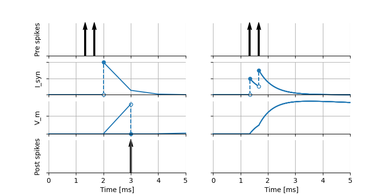
On the left, both pre-synaptic spikes are only processed at the end of the interval in which they occur. The statements in the update block are run every timestep for a fixed resolution of \(1~\text{ms}\), alternating with the statements in the onReceive handler for the spiking input port. Note that this means that the effect of the spikes becomes visible at the end of the timestep in \(I_\text{syn}\), but it takes another timestep before integrate_odes() is called again and consequently for the effect of the spikes to become visible in the membrane potential. This results in a threshold crossing and the neuron firing a spike. On the right half of the figure, the same presynaptic spike timing is used, but because events are processed at their exact time of occurrence. In this case, the update statements are called once to update the neuron from time 0 to \(1~\text{ms}\), then again to update from \(1~\text{ms}\) to the time of the first spike, then the spike is processed by running the statements in its onReceive block, then update is called to update from the time of the first spike to the second spike, and so on. The time courses of \(I_\text{syn}\) and \(V_\text{m}\) are such that the threshold is not reached and the neuron does not fire, illustrating the numerical differences that can occur when the same model is simulated using different strategies.

Guards

Variables which are defined in the state and parameters blocks can optionally be secured through guards. These guards are checked when the variable is assigned a value.

block:
    <declaration> [[<boolean_expression>]]

e.g.:

parameters:
    t_ref ms = 5 ms [[t_ref >= 0 ms]] # refractory period cannot be negative

References

[1]

Morrison A, Diesmann M (2008). Maintaining causality in discrete time neuronal network simulations. Lectures in Supercomputational Neurosciences: Dynamics in Complex Brain Networks, 267-278.

[2]

Stefan Rotter and Markus Diesmann. Exact digital simulation of time-invariant linear systems with applications to neuronal modeling. Biol. Cybern. 81, 381±402 (1999)