NESTML dopamine-modulated STDP synapse tutorial
Some text in this this notebook is copied verbatim from [1]. Network diagrams were modeled after [2].
Pavlov and Thompson (1902) first described classical conditioning: a phenomenon in which a biologically potent stimulus–the Unconditional Stimulus (UC)—is initially paired with a neutral stimulus—the Conditional Stimulus (CS). After many trials, learning is observed when the previously neutral stimuli start to elicit a response similar to that which was previously only elicited by the biologically potent stimulus. Pavlov and Thompson performed many experiments with dogs, observing their response (by monitoring salivation) to the appearance of a person who has been feeding them and the actual food appearing (UC). He demonstrated that the dogs started to salivate in the presence of the person who has been feeding them (or any other CS), rather than just when the food appears, because the CS had previously been associated with food.

Image credits: https://www.psychologicalscience.org/observer/revisiting-pavlovian-conditioning
In this tutorial, a dopamine-modulated STDP model is created in NESTML, and we characterize the model before using it in a network (reinforcement) learning task.
Model
Izhikevich (2007) revisits an important question: how does an animal know which of the many cues and actions preceding a reward should be credited for the reward? Izhikevich explains that dopamine-modulated STDP has a built-in instrumental conditioning property, i.e., the associations between cues, actions and rewards are learned automatically by reinforcing the firing patterns (networks of synapses) responsible, even when the firings of those patterns are followed by a delayed reward or masked by other network activity.
To achieve this, each synapse has an eligibility trace \(C\):
where \(\tau_C\) is the decay time constant of the eligibility trace and \(\text{STDP}(\Delta t)\) represents the magnitude of the change to make to the eligibility trace in response to a pair of pre- and post-synaptic spikes with temporal difference \(\Delta t = t_\text{post} − t_\text{pre}\). (This is just the usual STDP rule, see https://nestml.readthedocs.io/en/latest/tutorials/stdp_windows/stdp_windows.html.) Finally, \(\delta(t − t_\text{pre/post})\) is a Dirac delta function used to apply the effect of STDP to the trace at the times of pre- or post-synaptic spikes.
The concentration of dopamine is described by a variable \(D\):
where \(\tau_d\) is the time constant of dopamine re-absorption, \(D_c\) is a real number indicating the increase in dopamine concentration caused by each incoming dopaminergic spike; \(t_d^f\) are the times of these spikes.
Equations (1, 2) are then combined to calculate the change in synaptic strength \(W\):
When a post-synaptic spike arrives very shortly after a pre-synaptic spike, a standard STDP rule would immediately potentiate the synaptic strength. However, when using the three-factor STDP rule, this potentiation would instead be applied to the eligibility trace.
Because changes to the synaptic strength are gated by dopamine concentration \(D\) (Equation 3), changes are only made to the synaptic strength if \(D \neq 0\). Furthermore, if the eligibility trace has decayed back to 0 before any dopaminergic spikes arrive, the synaptic strength will also not be changed.
[1]:
%matplotlib inline

from typing import List, Optional

import matplotlib as mpl

mpl.rcParams["axes.formatter.useoffset"] = False
mpl.rcParams["axes.grid"] = True
mpl.rcParams["grid.color"] = "k"
mpl.rcParams["grid.linestyle"] = ":"
mpl.rcParams["grid.linewidth"] = 0.5
mpl.rcParams["figure.dpi"] = 120
mpl.rcParams["figure.figsize"] = [8., 3.]

import matplotlib.pyplot as plt
import nest
import numpy as np
import os
import random
import re

from pynestml.codegeneration.nest_code_generator_utils import NESTCodeGeneratorUtils
from pynestml.codegeneration.nest_tools import NESTTools
              -- N E S T --
  Copyright (C) 2004 The NEST Initiative

 Version: 3.8.0-post0.dev0
 Built: Dec 10 2024 12:04:47

 This program is provided AS IS and comes with
 NO WARRANTY. See the file LICENSE for details.

 Problems or suggestions?
   Visit https://www.nest-simulator.org

 Type 'nest.help()' to find out more about NEST.
Generating code with NESTML
To generate fast code, NESTML needs to process the synapse model together with the neuron model that will be its postsynaptic partner in the network instantiantion (see https://nestml.readthedocs.io/en/latest/nestml_language/synapses_in_nestml.html#generating-code).
In this tutorial, we will use a very simple integrate-and-fire model, where arriving spikes cause an instantaneous increment of the membrane potential, the “iaf_psc_delta” model.
When NESTML is invoked, the C++ code is generated for the models, and then built (compiled) as a NEST extension module, which is then loaded into the NEST kernel at runtime using nest.Install().
The resulting neuron and synapse model names are returned by the function, because when generating code for plastic synapses, there is typically a tight integration of the generated with code with that of the postsynaptic neuron model. For more information about this, please see the NESTML documentation section Generating code for plastic synapses. Hence, the resulting model names are
composed of associated neuron and synapse partners, because of the co-generation, for example, "stdp_synapse__with_iaf_psc_delta" and "iaf_psc_delta__with_stdp_synapse".
Formulating the model in NESTML
We now go on to define the full synapse model in NESTML:
[2]:
nestml_stdp_dopa_model = """
model neuromodulated_stdp_synapse:

    state:
        w real = 1.
        n real = 0.   # Neuromodulator concentration
        c real = 0.   # Eligibility trace
        pre_tr real = 0.
        post_tr real = 0.

    parameters:
        d ms = 1 ms
        tau_tr_pre ms = 20 ms   # STDP time constant for weight changes caused by pre-before-post spike pairings.
        tau_tr_post ms = 20 ms    # STDP time constant for weight changes caused by post-before-pre spike pairings.
        tau_c ms = 1000 ms    # Time constant of eligibility trace
        tau_n ms = 200 ms   # Time constant of dopaminergic trace
        b real = 0.   # Dopaminergic baseline concentration
        Wmax real = 200.    # Maximal synaptic weight
        Wmin real = 0.    # Minimal synaptic weight
        A_plus real = 1.    # Multiplier applied to weight changes caused by pre-before-post spike pairings. If b (dopamine baseline concentration) is zero, then A_plus is simply the multiplier for facilitation (as in the stdp_synapse model). If b is not zero, then A_plus will be the multiplier for facilitation only if n - b is positive, where n is the instantenous dopamine concentration in the volume transmitter. If n - b is negative, A_plus will be the multiplier for depression.
        A_minus real = 1.5    # Multiplier applied to weight changes caused by post-before-pre spike pairings. If b (dopamine baseline concentration) is zero, then A_minus is simply the multiplier for depression (as in the stdp_synapse model). If b is not zero, then A_minus will be the multiplier for depression only if n - b is positive, where n is the instantenous dopamine concentration in the volume transmitter. If n - b is negative, A_minus will be the multiplier for facilitation.
        A_vt real = 1.     # Multiplier applied to dopa spikes

    equations:
        pre_tr' = -pre_tr / tau_tr_pre
        post_tr' = -post_tr / tau_tr_post

    internals:
        tau_s 1/ms = (tau_c + tau_n) / (tau_c * tau_n)

    input:
        pre_spikes <- spike
        post_spikes <- spike
        mod_spikes <- spike

    output:
        spike

    onReceive(mod_spikes):
        n += A_vt / tau_n

    onReceive(post_spikes):
        post_tr += 1.

        # facilitation
        c += A_plus * pre_tr

    onReceive(pre_spikes):
        pre_tr += 1.

        # depression
        c -= A_minus * post_tr

        # deliver spike to postsynaptic partner
        emit_spike(w)

    # update from time t to t + timestep()
    update:
        integrate_odes()

        # timestep() returns the timestep to be made (in units of time)
        # the sequence here matters: the update step for w requires the "old" values of c and n
        w -= c * ( n / tau_s * expm1( -tau_s * timestep() ) \
                 - b * tau_c * expm1( -timestep() / tau_c ))
        w = max(0., w)
        c = c * exp(-timestep() / tau_c)
        n = n * exp(-timestep() / tau_n)
"""
Generate the code, build the user module and make the model available to instantiate in NEST:
[3]:
# generate and build code
module_name, neuron_model_name, synapse_model_name = \
    NESTCodeGeneratorUtils.generate_code_for("../../../models/neurons/iaf_psc_delta_neuron.nestml",
                                             nestml_stdp_dopa_model,
                                             post_ports=["post_spikes"],
                                             mod_ports=["mod_spikes"],
                                             logging_level="WARNING",
                                             codegen_opts={"weight_variable": {"neuromodulated_stdp_synapse": "w"}})
              -- N E S T --
  Copyright (C) 2004 The NEST Initiative

 Version: 3.8.0-post0.dev0
 Built: Dec 10 2024 12:04:47

 This program is provided AS IS and comes with
 NO WARRANTY. See the file LICENSE for details.

 Problems or suggestions?
   Visit https://www.nest-simulator.org

 Type 'nest.help()' to find out more about NEST.

[15,neuromodulated_stdp_synapse_nestml, WARNING, [12:8;12:17]]: Variable 'd' has the same name as a physical unit!
WARNING:Not preserving expression for variable "V_m" as it is solved by propagator solver
WARNING:Not preserving expression for variable "refr_t" as it is solved by propagator solver
WARNING:Not preserving expression for variable "V_m" as it is solved by propagator solver
WARNING:Not preserving expression for variable "refr_t" as it is solved by propagator solver
WARNING:Not preserving expression for variable "post_tr__for_neuromodulated_stdp_synapse_nestml" as it is solved by propagator solver
WARNING:Not preserving expression for variable "pre_tr" as it is solved by propagator solver
Running the simulation in NEST
Let’s define a function that will instantiate a simple network with one presynaptic cell and one postsynaptic cell connected by a single synapse, then run a simulation and plot the results.

[4]:
def run_network(pre_spike_time, post_spike_time, vt_spike_times,
                neuron_model_name,
                synapse_model_name,
                resolution=.1, # [ms]
                delay=1., # [ms]
                lmbda=1E-6,
                sim_time=None,  # if None, computed from pre and post spike times
                synapse_parameters=None,  # optional dictionary passed to the synapse
                fname_snip="",
                debug=False):

    nest.ResetKernel()
    NESTTools.set_nest_verbosity("ERROR")

    nest.print_time = False
    nest.Install(module_name)
    nest.resolution = resolution

    # create spike_generators with these times
    pre_sg = nest.Create("spike_generator",
                         params={"spike_times": [pre_spike_time]})
    post_sg = nest.Create("spike_generator",
                          params={"spike_times": [post_spike_time]})
    vt_sg = nest.Create("spike_generator",
                        params={"spike_times": vt_spike_times})

    # create  volume transmitter
    vt = nest.Create("volume_transmitter")
    vt_parrot = nest.Create("parrot_neuron")
    nest.Connect(vt_sg, vt_parrot)
    nest.Connect(vt_parrot, vt, syn_spec={"synapse_model": "static_synapse",
                                          "weight": 1.,
                                          "delay": 1.})   # delay is ignored!

    # set up custom synapse models
    wr = nest.Create("weight_recorder")
    nest.CopyModel(synapse_model_name, "stdp_nestml_rec",
                   {"weight_recorder": wr[0],
                    "w": 1.,
                    "delay": delay,
                    "receptor_type": 0,
                    "volume_transmitter": vt,
                    "tau_tr_pre": 10.})

    # create parrot neurons and connect spike_generators
    pre_neuron = nest.Create("parrot_neuron")
    post_neuron = nest.Create(neuron_model_name)

    spikedet_pre = nest.Create("spike_recorder")
    spikedet_post = nest.Create("spike_recorder")
    spikedet_vt = nest.Create("spike_recorder")

    #mm = nest.Create("multimeter", params={"record_from" : ["V_m"]})

    nest.Connect(pre_sg, pre_neuron, "one_to_one", syn_spec={"delay": 1.})
    nest.Connect(post_sg, post_neuron, "one_to_one", syn_spec={"delay": 1., "weight": 9999.})
    nest.Connect(pre_neuron, post_neuron, "all_to_all", syn_spec={"synapse_model": "stdp_nestml_rec"})
    #nest.Connect(mm, post_neuron)

    nest.Connect(pre_neuron, spikedet_pre)
    nest.Connect(post_neuron, spikedet_post)
    nest.Connect(vt_parrot, spikedet_vt)

    # get STDP synapse and weight before protocol
    syn = nest.GetConnections(source=pre_neuron, synapse_model="stdp_nestml_rec")
    if synapse_parameters is None:
        synapse_parameters = {}
    nest.SetStatus(syn, synapse_parameters)

    initial_weight = nest.GetStatus(syn)[0]["w"]
    np.testing.assert_allclose(initial_weight, 1)
    nest.Simulate(sim_time)
    updated_weight = nest.GetStatus(syn)[0]["w"]

    actual_t_pre_sp = nest.GetStatus(spikedet_pre)[0]["events"]["times"][0]
    actual_t_post_sp = nest.GetStatus(spikedet_post)[0]["events"]["times"][0]

    pre_spike_times_ = nest.GetStatus(spikedet_pre, "events")[0]["times"]
    assert len(pre_spike_times_) == 1 and pre_spike_times_[0] > 0

    post_spike_times_ = nest.GetStatus(spikedet_post, "events")[0]["times"]
    assert len(post_spike_times_) == 1 and post_spike_times_[0] > 0

    vt_spike_times_ = nest.GetStatus(spikedet_vt, "events")[0]["times"]
    assert len(vt_spike_times_) == 1 and vt_spike_times_[0] > 0

    #dt = actual_t_post_sp - actual_t_pre_sp
    dt = 0.
    dw = updated_weight

    return dt, dw
[5]:
def run_vt_spike_timing_experiment(neuron_model_name, synapse_model_name, synapse_parameters=None):
    sim_time = 10000.    # [ms] -- make sure to simulate for much longer than the eligibility trace
                         #         time constant, which is typically the slowest time constant in
                         #         the system, PLUS the time of the latest vt spike
    pre_spike_time = 1.  # [ms]
    post_spike_time = 3. # [ms]
    delay = .5           # dendritic delay [ms]

    dt_vec = []
    dw_vec = []
    for vt_spike_time in np.round(np.linspace(4, 5000, 12)).astype(float):  # sim_time - 10 * delay
        dt, dw = run_network(pre_spike_time, post_spike_time, [vt_spike_time],
                          neuron_model_name,
                          synapse_model_name,
                          delay=delay, # [ms]
                          synapse_parameters=synapse_parameters,
                          sim_time=sim_time)
        dt_vec.append(vt_spike_time)
        dw_vec.append(dw)

    return dt_vec, dw_vec, delay
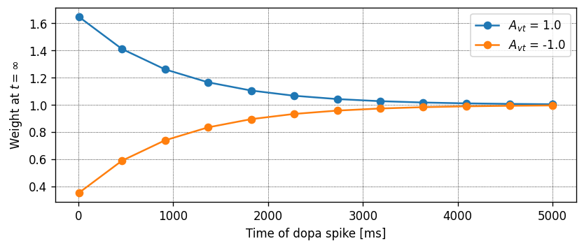
[6]:
fig, ax = plt.subplots()
for A_vt in [1., -1.]:
    dt_vec, dw_vec, delay = run_vt_spike_timing_experiment(neuron_model_name,
                                                       synapse_model_name,
                                                       synapse_parameters={"A_vt": A_vt})
    ax.plot(dt_vec, dw_vec, marker="o", label="$A_{vt}$ = " + str(A_vt))

ax.set_xlabel("Time of dopa spike [ms]")
ax.set_ylabel("Weight at $t = \infty$")
ax.legend()
plt.show()
plt.close(fig)
[6]:
<matplotlib.legend.Legend at 0x7f35d539a710>
Learning through dopamine
In this section we simulate the spiking activity of a group of neurons with the learning rule as described above. Here, we perform the simulation on 10 iaf_psc_delta neurons in which each of the neurons receives input from an independent Poisson source of 50Hz. These neurons are also connected to a single dopamine spike source. These dopamine spikes are delivered to the neurons as reward and punishment signals at specific time intervals.

Single dopamine source, multiple independent pre-post cell pairs (3 pairs shown).
[7]:
# Labels for x and y axes for traces used in plotting functions
labels = {"c": {"x_label": "Times [ms]", "y_label": "Eligibility \ntrace (c)"},
          "w": {"x_label": "Times [ms]", "y_label": "Weight \ntrace (w)"},
          "pre_tr": {"x_label": "Times [ms]", "y_label": "Presynaptic \ntrace (pre_tr)"},
          "n": {"x_label": "Times [ms]", "y_label": "Dopamine \ntrace (n)"}
         }
[8]:
# Plot trace values for a neurons or set of neurons
def plot_traces_for_neuron(log, recordables, neuron_numbers=None, pos_dopa_spike_times=None, neg_dopa_spike_times=None):
    """
    Plots the trace values for the given list of neuron IDs
    """
    times = log["t"]
    trace_values = {}
    # Initialize the list if "neuron_numbers" is None, which corresponds to all neurons
    if neuron_numbers is None:
        neuron_numbers = np.array([i+1 for i in range(10)])

    # The actual neuron numbers are -1 of the given numbers
    neuron_numbers_actual = np.array(neuron_numbers) - 1

    # Get the values of recordables for the given neuron IDs
    for recordable in recordables:
        trace_values[recordable] = np.array(log[recordable])[:, neuron_numbers_actual]

    n_neurons = len(neuron_numbers)
    palette = plt.get_cmap("tab10")

    for i in range(n_neurons):
        fig, ax = plt.subplots(nrows=len(recordables), sharex=True, squeeze=False)
        ax = ax.flatten()
        fig.suptitle("Trace values for Neuron " + str(neuron_numbers[i]))
        for j, recordable in enumerate(recordables):
            ax[j].plot(times, trace_values[recordable][:, i], label="neuron " + str(neuron_numbers[i]), color=palette(neuron_numbers_actual[i]))
            ax[j].set_xlim(xmin=0)
            ax[j].set_ylabel(labels[recordable]["y_label"], rotation=0, ha="right", va="center")
            ax[j].legend(loc="upper right", labelspacing=0.)
            if pos_dopa_spike_times is not None:
                ax[j].scatter(pos_dopa_spike_times, np.ones_like(pos_dopa_spike_times) * np.amin(trace_values[recordable][:, i]), marker="^", c="green", s=20)
            if neg_dopa_spike_times is not None:
                ax[j].scatter(neg_dopa_spike_times, np.ones_like(neg_dopa_spike_times) * np.amin(trace_values[recordable][:, i]), marker="^", c="red", s=20)
        fig.tight_layout(rect=[0, 0.03, 1, 0.95])
        plt.show()
        plt.close(fig)
[9]:
def plot_spiking_activity(neuron_spike_times, pos_dopa_spike_times, neg_dopa_spike_times, source_ids, total_t_sim):
    fig, ax = plt.subplots()
    palette = plt.get_cmap("tab10")

    n_neurons = len(neuron_spike_times)
    y_ticks = [i * 10 for i in range(n_neurons, 0, -1)]
    for i in range(n_neurons):
        ax.scatter(neuron_spike_times[i], np.ones_like(neuron_spike_times[i]) * y_ticks[i], color=palette(i), s=1)

    if pos_dopa_spike_times is not None:
        ax.scatter(pos_dopa_spike_times, np.zeros_like(pos_dopa_spike_times), marker="^", c="green", s=100)
    if neg_dopa_spike_times is not None:
        ax.scatter(neg_dopa_spike_times, np.zeros_like(pos_dopa_spike_times), marker="^", c="red", s=100)

    ax.set_xlim(0., total_t_sim)
    ax.set_ylim(ymin=0)
    ax.set_xlim(xmin=0)
    ax.set_yticks(y_ticks)
    ax.set_yticklabels(source_ids)
    ax.set_xlabel("Time [ms]")
    ax.set_ylabel("Neuron ID")
    plt.tight_layout()
    plt.show()
    plt.close(fig)
Here, we setup the network with 10 neurons each connected to a Poisson source. The neurons are also connected to a volume transmitter that acts as a dopamine spike source.
[10]:
# simulation parameters
resolution = .1

# network parameters
n_neurons = 10
tau_n = 50.
tau_c = 100.
pre_poisson_rate = 50.  # [s^-1]
initial_weight = 5.6  # controls initial firing rate before potentiation

# stimulus parameters
pos_dopa_spike_times = [2000, 3000, 4000]
neg_dopa_spike_times = [8000, 9000, 10000]
A_vt = [10., -10.]

nest.ResetKernel()
NESTTools.set_nest_verbosity("ERROR")

nest.print_time = False
nest.Install(module_name)
nest.resolution = resolution

# Create the neurons
neurons = nest.Create(neuron_model_name, n_neurons)

# Create a poisson generator
poisson_gen = nest.Create("poisson_generator", n_neurons, params={"rate": pre_poisson_rate})
parrot_neurons = nest.Create("parrot_neuron", n_neurons)

# Spike generators
vt_sg = nest.Create("spike_generator", params={"spike_times": pos_dopa_spike_times + neg_dopa_spike_times})

# Spike recorder
spike_rec = nest.Create("spike_recorder")
spike_rec_vt = nest.Create("spike_recorder")
spike_re_pt = nest.Create("spike_recorder")

# create  volume transmitter
vt = nest.Create("volume_transmitter")
vt_parrot = nest.Create("parrot_neuron")
nest.Connect(vt_sg, vt_parrot, syn_spec={"weight": -1.})
nest.Connect(vt_parrot, vt, syn_spec={"synapse_model": "static_synapse",
                                      "weight": 1.,
                                      "delay": 1.})

# multimeters
mms = [nest.Create("multimeter", params= {"record_from": ["V_m"]}) for _ in range(n_neurons)]

# set up custom synapse models
wr = nest.Create("weight_recorder")
nest.CopyModel(synapse_model_name, "stdp_nestml_rec",
            {"weight_recorder": wr[0],
             "w": initial_weight,
             "delay": delay,
             "receptor_type": 0,
             "volume_transmitter": vt,
             "tau_n": tau_n,
             "tau_c": tau_c,
            })

# Connect everything
nest.Connect(poisson_gen, parrot_neurons, "one_to_one")
nest.Connect(parrot_neurons, neurons, "one_to_one", syn_spec="stdp_nestml_rec")

nest.Connect(neurons, spike_rec)
nest.Connect(vt_parrot, spike_rec_vt)

for i in range(n_neurons):
    nest.Connect(mms[i], neurons[i])
This is a helper function that runs the simulation in chunks of time intervals and records the values of the synapse properties passed as recordables.
[11]:
def run_simulation_in_chunks(sim_chunks, sim_time, recordables, neurons):
    sim_time_per_chunk = sim_time / sim_chunks

    # Init log to collect the values of all recordables
    log = {}
    log["t"] = []

    # Initialize all the arrays
    # Additional one entry is to store the trace value before the simulation begins
    for rec in recordables:
        log[rec] = (sim_chunks + 1) * [[]]

    # Get the value of trace values before the simulation
    syn = nest.GetConnections(target=neurons, synapse_model="stdp_nestml_rec")
    for rec in recordables:
        log[rec][0] = syn.get(rec)

    log["t"].append(nest.GetKernelStatus("biological_time"))

    # Run the simulation in chunks
    nest.Prepare()
    for i in range(sim_chunks):
        print(str(i) + " out of " + str(sim_chunks))
        # Set the reward / punishment for dopa spikes
        # Set the punishment signal only when the timed during simulation == the first negative dopa spike time
        # Otherwise set the reward signal
        sim_start_time = i * sim_time_per_chunk
        sim_end_time = sim_start_time + sim_time_per_chunk

        if sim_end_time > neg_dopa_spike_times[0]:
            syn.set({"A_vt": A_vt[1]})
        else:
            syn.set({"A_vt": A_vt[0]})

        nest.Run(sim_time//sim_chunks)

        # log current values
        log["t"].append(nest.GetKernelStatus("biological_time"))

        # Get the value of trace after the simulation
        for rec in recordables:
            log[rec][i + 1] = syn.get(rec)
    nest.Cleanup()

    return log
Run simulation in NEST
Let’s run the simulation and record the neuron spike times and synapse parameters like the eligibility trace c, the presynaptic trace pre_tr, the dopamine trace n, and the weight w.
[12]:
# Run simulation
sim_time = 12000
n_chunks = 400
recordables = ["c", "pre_tr", "n", "w"]
log = run_simulation_in_chunks(n_chunks, sim_time, recordables, neurons)

times = spike_rec.get("events")["times"]
senders = spike_rec.get("events")["senders"]

times_vt = spike_rec_vt.get("events")["times"]

connections = nest.GetConnections(neurons)
source_ids = connections.get("source")  # source IDs of all neurons
source_ids = list(set(source_ids))

neuron_spike_times = [[] for _ in range(n_neurons)]
for i in range(n_neurons):
    neuron_spike_times[i] = times[senders == source_ids[i]]
0 out of 400
1 out of 400
2 out of 400
3 out of 400
4 out of 400
5 out of 400
6 out of 400
7 out of 400
8 out of 400
9 out of 400
10 out of 400
11 out of 400
12 out of 400
13 out of 400
14 out of 400
15 out of 400
16 out of 400
17 out of 400
18 out of 400
19 out of 400
20 out of 400
21 out of 400
22 out of 400
23 out of 400
24 out of 400
25 out of 400
26 out of 400
27 out of 400
28 out of 400
29 out of 400
30 out of 400
31 out of 400
32 out of 400
33 out of 400
34 out of 400
35 out of 400
36 out of 400
37 out of 400
38 out of 400
39 out of 400
40 out of 400
41 out of 400
42 out of 400
43 out of 400
44 out of 400
45 out of 400
46 out of 400
47 out of 400
48 out of 400
49 out of 400
50 out of 400
51 out of 400
52 out of 400
53 out of 400
54 out of 400
55 out of 400
56 out of 400
57 out of 400
58 out of 400
59 out of 400
60 out of 400
61 out of 400
62 out of 400
63 out of 400
64 out of 400
65 out of 400
66 out of 400
67 out of 400
68 out of 400
69 out of 400
70 out of 400
71 out of 400
72 out of 400
73 out of 400
74 out of 400
75 out of 400
76 out of 400
77 out of 400
78 out of 400
79 out of 400
80 out of 400
81 out of 400
82 out of 400
83 out of 400
84 out of 400
85 out of 400
86 out of 400
87 out of 400
88 out of 400
89 out of 400
90 out of 400
91 out of 400
92 out of 400
93 out of 400
94 out of 400
95 out of 400
96 out of 400
97 out of 400
98 out of 400
99 out of 400
100 out of 400
101 out of 400
102 out of 400
103 out of 400
104 out of 400
105 out of 400
106 out of 400
107 out of 400
108 out of 400
109 out of 400
110 out of 400
111 out of 400
112 out of 400
113 out of 400
114 out of 400
115 out of 400
116 out of 400
117 out of 400
118 out of 400
119 out of 400
120 out of 400
121 out of 400
122 out of 400
123 out of 400
124 out of 400
125 out of 400
126 out of 400
127 out of 400
128 out of 400
129 out of 400
130 out of 400
131 out of 400
132 out of 400
133 out of 400
134 out of 400
135 out of 400
136 out of 400
137 out of 400
138 out of 400
139 out of 400
140 out of 400
141 out of 400
142 out of 400
143 out of 400
144 out of 400
145 out of 400
146 out of 400
147 out of 400
148 out of 400
149 out of 400
150 out of 400
151 out of 400
152 out of 400
153 out of 400
154 out of 400
155 out of 400
156 out of 400
157 out of 400
158 out of 400
159 out of 400
160 out of 400
161 out of 400
162 out of 400
163 out of 400
164 out of 400
165 out of 400
166 out of 400
167 out of 400
168 out of 400
169 out of 400
170 out of 400
171 out of 400
172 out of 400
173 out of 400
174 out of 400
175 out of 400
176 out of 400
177 out of 400
178 out of 400
179 out of 400
180 out of 400
181 out of 400
182 out of 400
183 out of 400
184 out of 400
185 out of 400
186 out of 400
187 out of 400
188 out of 400
189 out of 400
190 out of 400
191 out of 400
192 out of 400
193 out of 400
194 out of 400
195 out of 400
196 out of 400
197 out of 400
198 out of 400
199 out of 400
200 out of 400
201 out of 400
202 out of 400
203 out of 400
204 out of 400
205 out of 400
206 out of 400
207 out of 400
208 out of 400
209 out of 400
210 out of 400
211 out of 400
212 out of 400
213 out of 400
214 out of 400
215 out of 400
216 out of 400
217 out of 400
218 out of 400
219 out of 400
220 out of 400
221 out of 400
222 out of 400
223 out of 400
224 out of 400
225 out of 400
226 out of 400
227 out of 400
228 out of 400
229 out of 400
230 out of 400
231 out of 400
232 out of 400
233 out of 400
234 out of 400
235 out of 400
236 out of 400
237 out of 400
238 out of 400
239 out of 400
240 out of 400
241 out of 400
242 out of 400
243 out of 400
244 out of 400
245 out of 400
246 out of 400
247 out of 400
248 out of 400
249 out of 400
250 out of 400
251 out of 400
252 out of 400
253 out of 400
254 out of 400
255 out of 400
256 out of 400
257 out of 400
258 out of 400
259 out of 400
260 out of 400
261 out of 400
262 out of 400
263 out of 400
264 out of 400
265 out of 400
266 out of 400
267 out of 400
268 out of 400
269 out of 400
270 out of 400
271 out of 400
272 out of 400
273 out of 400
274 out of 400
275 out of 400
276 out of 400
277 out of 400
278 out of 400
279 out of 400
280 out of 400
281 out of 400
282 out of 400
283 out of 400
284 out of 400
285 out of 400
286 out of 400
287 out of 400
288 out of 400
289 out of 400
290 out of 400
291 out of 400
292 out of 400
293 out of 400
294 out of 400
295 out of 400
296 out of 400
297 out of 400
298 out of 400
299 out of 400
300 out of 400
301 out of 400
302 out of 400
303 out of 400
304 out of 400
305 out of 400
306 out of 400
307 out of 400
308 out of 400
309 out of 400
310 out of 400
311 out of 400
312 out of 400
313 out of 400
314 out of 400
315 out of 400
316 out of 400
317 out of 400
318 out of 400
319 out of 400
320 out of 400
321 out of 400
322 out of 400
323 out of 400
324 out of 400
325 out of 400
326 out of 400
327 out of 400
328 out of 400
329 out of 400
330 out of 400
331 out of 400
332 out of 400
333 out of 400
334 out of 400
335 out of 400
336 out of 400
337 out of 400
338 out of 400
339 out of 400
340 out of 400
341 out of 400
342 out of 400
343 out of 400
344 out of 400
345 out of 400
346 out of 400
347 out of 400
348 out of 400
349 out of 400
350 out of 400
351 out of 400
352 out of 400
353 out of 400
354 out of 400
355 out of 400
356 out of 400
357 out of 400
358 out of 400
359 out of 400
360 out of 400
361 out of 400
362 out of 400
363 out of 400
364 out of 400
365 out of 400
366 out of 400
367 out of 400
368 out of 400
369 out of 400
370 out of 400
371 out of 400
372 out of 400
373 out of 400
374 out of 400
375 out of 400
376 out of 400
377 out of 400
378 out of 400
379 out of 400
380 out of 400
381 out of 400
382 out of 400
383 out of 400
384 out of 400
385 out of 400
386 out of 400
387 out of 400
388 out of 400
389 out of 400
390 out of 400
391 out of 400
392 out of 400
393 out of 400
394 out of 400
395 out of 400
396 out of 400
397 out of 400
398 out of 400
399 out of 400
Spiking activity
[13]:
# Plot the spiking activity
plot_spiking_activity(neuron_spike_times, pos_dopa_spike_times, neg_dopa_spike_times, source_ids, sim_time)
/tmp/ipykernel_1318730/670906053.py:23: UserWarning:FigureCanvasAgg is non-interactive, and thus cannot be shown
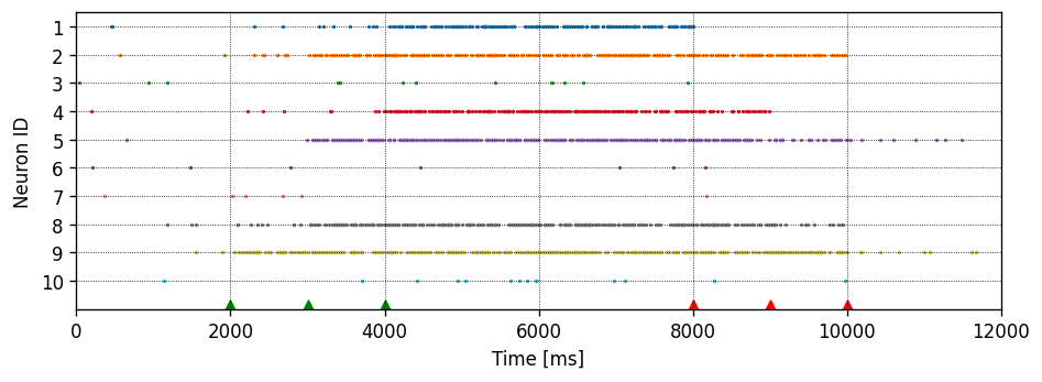
From the spiking activity of the neurons, we can see that the firing rate of the neurons increases after the dopamine spikes or reward signals (green triangles in the plot) are applied to the synapses. Consequently, when the punishment signals are applied (red triangles), the firing rate decreases. In order to understand the dynamics, let’s plot the different trace variables of the synapse.
Plot the trace values
Let’s plot the trace values and the weight for each synapse. Note that the dopamine trace is the same for every synapse.
[14]:
# Plot trace values for all neurons
plot_traces_for_neuron(log, ["c", "w", "n"], pos_dopa_spike_times=pos_dopa_spike_times, neg_dopa_spike_times=neg_dopa_spike_times)
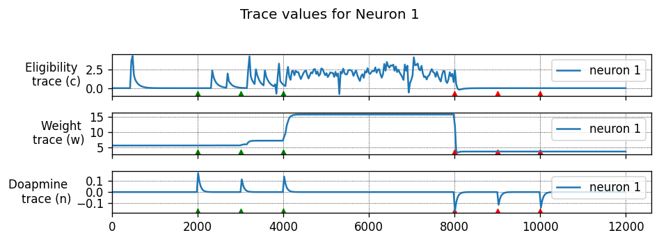
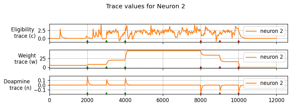
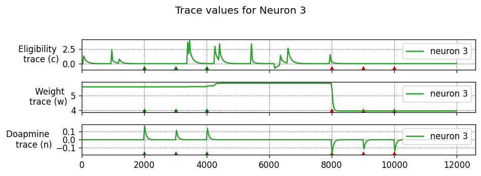
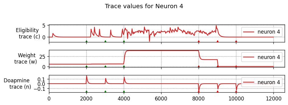
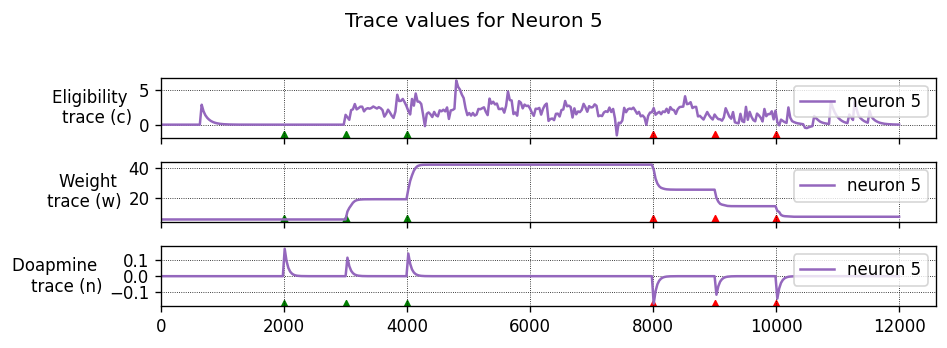
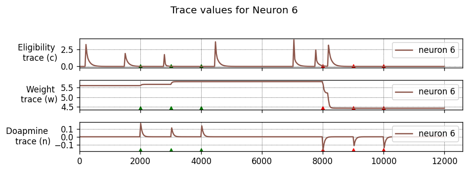
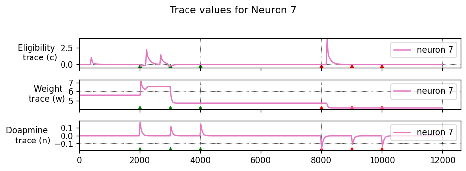
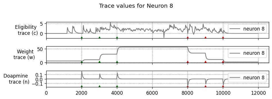
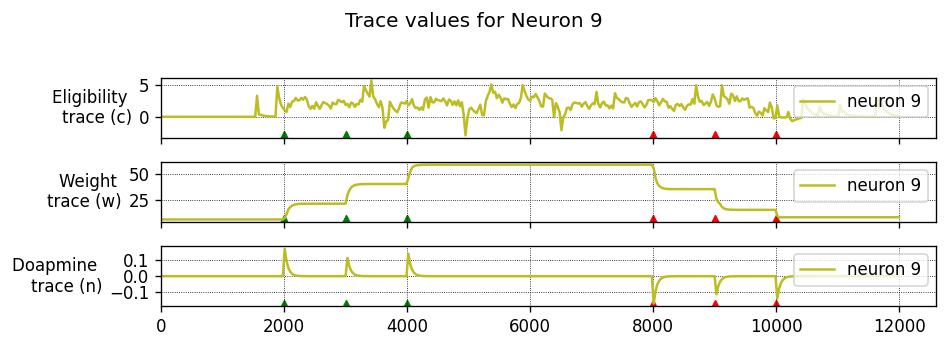
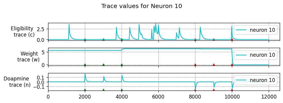
As we can see, the eligibility trace values for neurons 1, 2, 4, 5, and 9 are large when the dopamine spikes are applied, which increases the weights of these neurons, resulting in stronger firing. If the dopamine spikes arrive while the eligibility trace is close to zero, the weight does not increase or increases only very little.
In our simulation above, we set a low value of 50 ms for the time constant of the dopamine trace \(\tau_n\). This means that the dopamine signal does not sustain for a long time, allowing only some neurons that fire around the time when the dopamine spikes (reward signal) are applied have their synapses strengthened (see the weight trace plots) and consequenty increase their firing rate. Similarly, the firing rate is decreased when the dopamine spikes (punishment signals) are applied. For neuron 9, the punishment signal doesn’t seem to affect the firing rate. This behavior can be explained by the time constant of the signals and the very large weights after the initial potentiation, resulting in sustained firing.
Play around with the initial weight value w and dopamine time constant \(\tau_n\) to simulate and see the effects of these values on firing rates and trace values.
Noisy Cue-Association: Temporal Credit-Assignment Task
In this experiment, the synapse is embedded in a network consisting of 800 excitatory, and 200 inhibitory neurons, that are randomly and sparsely connected. The network is in the balanced state, meaning that excitatory currents are roughly matched in mean amplitude over time, and the neurons have a membrane potential close to the firing threshold, firing only sparsely and with statistics approaching that of a Poisson process [4].
Using this network, we illustrate a classical (Pavlovian) conditioning experiment: rewarding a conditioned stimulus \(S_1\) embedded in a continuous stream of irrelevant but equally salient stimuli [3]. The conditioned stimulus is repeatedly presented to the network, causing a transient of activity against the background of low-rate random background firing. The CS is always followed by a reward, which reinforces the recurrent excitatory pathways in the network.
To simulate the experiment, n_subgroups random sets of neurons (each representing stimulus \(S_1\) through \(S_\text{n\_subgroups}\)) are chosen from the pool of excitatory and inhibitory neurons in the network. To present a stimulus to the network, we create n_subgroups spike generators (named stim_sg), and connect each to its individual target group of subgroup_size neurons in the network (here, 50) with a very large weight, so that the stimulus spike generator firing
will cause all of the neurons in the subgroup to fire.
A continuous input stream is generated, consisting of stimuli \(S_i (1 \leq i \leq \text{n\_subgroups})\) in a random order with random intervals of rate stimulus_rate and at least min_stimulus_presentation_delay. After every presentation of the CS (\(S_1\)), a reward in the form of an increase of extra-cellular dopamine is delivered to all plastic synapses in the network, after a random delay between min_dopa_reinforcement_delay and max_dopa_reinforcement_delay. These
delays were chosen lower than in the original publications ([1], [3]) to keep the simulation times low for this interactive tutorial. The delay is large enough to allow irrelevant input stimuli to be presented during the waiting period; these can be considered as distractors.
At the beginning of the experiment the neurons representing each stimulus \(S_i\) respond equally. However, after many trials, the network starts to show reinforced response to the CS (\(S_1\)). Because synapses coming out of neurons representing \(S_1\) are always tagged with the eligibility trace when the reward is delivered, whereas the synapses connected to neurons representing irrelevant stimuli will only be occasionally tagged, the average strength of synaptic connections from neurons representing stimulus \(S_1\) becomes stronger than the mean synaptic connection strength in the rest of the network. Therefore, the other neurons in the network learn to listen more closely to the stimulus \(S_1\), because the activation of this pathway causes a reward.

This network uses neurons with a decaying-exponential shaped postsynaptic current. Let’s first generate the code for those.
[15]:
# generate and build code

module_name, neuron_model_name, synapse_model_name = \
    NESTCodeGeneratorUtils.generate_code_for("../../../models/neurons/iaf_psc_exp_neuron.nestml",
                                             nestml_stdp_dopa_model,
                                             post_ports=["post_spikes"],
                                             mod_ports=["mod_spikes"],
                                             logging_level="WARNING",
                                             codegen_opts={"weight_variable": {"neuromodulated_stdp_synapse": "w"}})
              -- N E S T --
  Copyright (C) 2004 The NEST Initiative

 Version: 3.8.0-post0.dev0
 Built: Dec 10 2024 12:04:47

 This program is provided AS IS and comes with
 NO WARRANTY. See the file LICENSE for details.

 Problems or suggestions?
   Visit https://www.nest-simulator.org

 Type 'nest.help()' to find out more about NEST.

[15,neuromodulated_stdp_synapse_nestml, WARNING, [12:8;12:17]]: Variable 'd' has the same name as a physical unit!
WARNING:Under certain conditions, the propagator matrix is singular (contains infinities).
WARNING:List of all conditions that result in a singular propagator:
WARNING:        tau_m = tau_syn_exc
WARNING:        tau_m = tau_syn_inh
WARNING:Not preserving expression for variable "I_syn_exc" as it is solved by propagator solver
WARNING:Not preserving expression for variable "I_syn_inh" as it is solved by propagator solver
WARNING:Not preserving expression for variable "V_m" as it is solved by propagator solver
WARNING:Not preserving expression for variable "refr_t" as it is solved by propagator solver
WARNING:Not preserving expression for variable "post_tr__for_neuromodulated_stdp_synapse_nestml" as it is solved by propagator solver
WARNING:Not preserving expression for variable "pre_tr" as it is solved by propagator solver
Now, we define the network and the simulation parameters.
[16]:
# simulation parameters

dt = .1    # the resolution in ms
delay = 1.    # synaptic delay in ms
total_t_sim = 10000.  # [ms]

# parameters for balanced network

g = 4.  # ratio inhibitory weight/excitatory weight
epsilon = .1  # connection probability
NE = 800  # number of excitatory neurons
NI = 200  # number of inhibitory neurons
N_neurons = NE + NI   # number of neurons in total
N_rec = 50      # record from 50 neurons

CE = int(epsilon * NE)  # number of excitatory synapses per neuron
CI = int(epsilon * NI)  # number of inhibitory synapses per neuron
C_tot = int(CI + CE)      # total number of synapses per neuron

# neuron parameters

tauSyn = 1.  # synaptic time constant [ms]
tauMem = 10.  # time constant of membrane potential [ms]
CMem = 300.  # capacitance of membrane [pF]

neuron_params_exc = {"C_m": CMem,
                     "tau_m": tauMem,
                     "tau_syn_exc": tauSyn,
                     "tau_syn_inh": tauSyn,
                     "refr_T": 4.0,
                     "E_L": -65.,
                     "V_reset": -70.,
                     "V_m": -65.,
                     "V_th": -55.4,
                     "I_e": 0.}   # [pA]

neuron_params_inh = {"C_m": CMem,
                     "tau_m": tauMem,
                     "tau_syn_exc": tauSyn,
                     "tau_syn_inh": tauSyn,
                     "refr_T": 2.0,
                     "E_L": -65.,
                     "V_reset": -70.,
                     "V_m": -65.,
                     "V_th": -56.4}

# J_ex should be large enough so that when stimulus excites the subgroup cells,
# the subgroup cells cause an excitatory transient in the network to establish
# a causal STDP timing and positive eligibility trace in the synapses
J_ex = 300.  # amplitude of excitatory postsynaptic current
J_in = -g * J_ex    # amplitude of inhibitory postsynaptic current
J_poisson = 2500.
J_stim = 5000.

p_rate = 5.    # external Poisson generator rate [s^-1]

# synapse parameters

learning_rate = .1   # multiplier for weight updates
tau_c = 200.  # [ms]
tau_n = 200.  # [ms]

# stimulus parameters

n_subgroups = 2  # = n_stimuli
subgroup_size = 50   # per subgroup, this many neurons are stimulated when stimulus is presented
reinforced_subgroup_idx = 0
stimulus_rate = 5.   # [s^-1]

min_stimulus_presentation_delay = 10.   # minimum time between presenting stimuli [ms]

min_dopa_reinforcement_delay = 10. # [ms]
max_dopa_reinforcement_delay = 30. # [ms]
With the parameters defined, we are ready to instantiate and connect the network.
[17]:
nest.ResetKernel()
NESTTools.set_nest_verbosity("ERROR")
nest.print_time = False
nest.Install(module_name)    # load dynamic library (NEST extension module) into NEST kernel
nest.local_num_threads = 1
nest.resolution = dt
nest.overwrite_files = True

nodes_ex = nest.Create(neuron_model_name, NE, params=neuron_params_exc)
nodes_in = nest.Create(neuron_model_name, NI, params=neuron_params_inh)
noise = nest.Create("poisson_generator", params={"rate": p_rate})
vt_spike_times = []
vt_sg = nest.Create("spike_generator",
                    params={"spike_times": vt_spike_times,
                            "allow_offgrid_times": True})

espikes = nest.Create("spike_recorder")
ispikes = nest.Create("spike_recorder")
spikedet_vt = nest.Create("spike_recorder")

# create volume transmitter
vt = nest.Create("volume_transmitter")
vt_parrot = nest.Create("parrot_neuron")
nest.Connect(vt_sg, vt_parrot)
nest.Connect(vt_parrot, vt, syn_spec={"synapse_model": "static_synapse",
                                      "weight": 1.,
                                      "delay": 1.})   # delay is ignored
# set up custom synapse models
wr = nest.Create("weight_recorder")
nest.CopyModel(synapse_model_name, "excitatory",
               {"weight_recorder": wr, "w": J_ex, "delay": delay, "receptor_type": 0,
                "volume_transmitter": vt, "A_plus": learning_rate * 1., "A_minus": learning_rate * 1.5,
               "tau_n": tau_n,
               "tau_c": tau_c})

nest.CopyModel("static_synapse", "inhibitory",
               {"weight": J_in, "delay": delay})
nest.CopyModel("static_synapse", "poisson",
               {"weight": J_poisson, "delay": delay})

# make subgroups: pick from excitatory population. subgroups can overlap, but
# each group consists of `subgroup_size` unique neurons

subgroup_indices = n_subgroups * [[]]
for i in range(n_subgroups):
    ids_nonoverlapping = False
    # TODO: replace while loop with:
    # subgroup_indices[i] = np.sort(np.random.choice(NE, size=subgroup_size, replace=False))
    while not ids_nonoverlapping:
        ids = np.random.randint(0, NE, subgroup_size)
        ids_nonoverlapping = len(np.unique(ids)) == subgroup_size
    ids.sort()
    subgroup_indices[i] = ids

# make one spike generator and one parrot neuron for each subgroup
stim_sg = nest.Create("spike_generator", n_subgroups)
stim_parrots = nest.Create("parrot_neuron", n_subgroups)

# make recording devices
stim_spikes_rec = nest.Create("spike_recorder")
mm = nest.Create("multimeter", params={"record_from": ["V_m"], "interval": dt})
mms = [nest.Create("multimeter", params={"record_from": ["V_m"], "interval": dt}) for _ in range(10)]

# connect everything up
nest.Connect(stim_parrots, stim_spikes_rec, syn_spec="static_synapse")
nest.Connect(noise, nodes_ex + nodes_in, syn_spec="poisson")
nest.Connect(mm, nodes_ex[0])
[nest.Connect(mms[i], nodes_ex[i]) for i in range(10)]

nest.Connect(stim_sg, stim_parrots, "one_to_one")

for i in range(n_subgroups):
    nest.Connect(stim_parrots[i], nodes_ex[subgroup_indices[i]], "all_to_all", syn_spec={"weight": J_stim})

conn_params_ex = {"rule": "fixed_indegree", "indegree": CE}
nest.Connect(nodes_ex, nodes_ex + nodes_in, conn_params_ex, "excitatory")

conn_params_in = {"rule": "fixed_indegree", "indegree": CI}
nest.Connect(nodes_in, nodes_ex + nodes_in, conn_params_in, "inhibitory")

nest.Connect(vt_parrot, spikedet_vt)

nest.Connect(nodes_ex, espikes, syn_spec="static_synapse")
nest.Connect(nodes_in, ispikes, syn_spec="static_synapse")

# generate stimulus timings (input stimulus and reinforcement signal)

t_dopa_spikes = []
t_pre_sg_spikes = [[] for _ in range(n_subgroups)]   # mapping from subgroup_idx to a list of spike (or presentation) times of that subgroup

t = 0.   # [ms]
ev_timestamps = []
while t < total_t_sim:
    # jump to time of next stimulus presentation
    dt_next_stimulus = max(min_stimulus_presentation_delay, np.round(random.expovariate(stimulus_rate) * 1000)) # [ms]
    t += dt_next_stimulus

    ev_timestamps.append(t)

    # apply stimulus
    subgroup_idx = np.random.randint(0, n_subgroups)
    t_pre_sg_spikes[subgroup_idx].append(t)

    # reinforce?
    if subgroup_idx == reinforced_subgroup_idx:
        # fire a dopa spike some time after the current time
        t_dopa_spike = t + min_dopa_reinforcement_delay + np.random.randint(max_dopa_reinforcement_delay - min_dopa_reinforcement_delay)
        t_dopa_spikes.append(t_dopa_spike)

print("--> Stimuli will be presented at times: " + str(ev_timestamps))

# set the spike times in the spike generators
for i in range(n_subgroups):
    t_pre_sg_spikes[i].sort()
    stim_sg[i].spike_times = t_pre_sg_spikes[i]

t_dopa_spikes.sort()
vt_sg.spike_times = t_dopa_spikes

print("--> t_dopa_spikes = " + str(t_dopa_spikes))
--> Stimuli will be presented at times: [330.0, 650.0, 1810.0, 2036.0, 2097.0, 2127.0, 2209.0, 2631.0, 2843.0, 3094.0, 3157.0, 3358.0, 3432.0, 4050.0, 4176.0, 4227.0, 4573.0, 4830.0, 4973.0, 5166.0, 5406.0, 5638.0, 5723.0, 5770.0, 5780.0, 5833.0, 6078.0, 6312.0, 6509.0, 6764.0, 7036.0, 7222.0, 7242.0, 7264.0, 7445.0, 7984.0, 8092.0, 8475.0, 8534.0, 8621.0, 8947.0, 9003.0, 9049.0, 9068.0, 9121.0, 9395.0, 9444.0, 9473.0, 9576.0, 9727.0, 9796.0, 10262.0]
--> t_dopa_spikes = [344.0, 1825.0, 2064.0, 2234.0, 2856.0, 3460.0, 4066.0, 4197.0, 4242.0, 4598.0, 4998.0, 5665.0, 5744.0, 5792.0, 5853.0, 6107.0, 6332.0, 6533.0, 7239.0, 7256.0, 7464.0, 8963.0, 9016.0, 9073.0, 9416.0, 9454.0, 9484.0, 9589.0, 9810.0, 10288.0]
Run the simulation. Instead of just running from start to finish in one go:
[18]:
# nest.Simulate(total_t_sim)
we split the simulation into equally-sized chunks, so that we can measure and record the state of some internal variables inbetween:
[19]:
def run_chunked_simulation(n_chunks, all_nodes, reinforced_group_nodes, not_reinforced_group_nodes):
    # init log
    log = {}
    log["t"] = []
    log["w_net"] = []
    recordables = ["c_sum", "w_avg", "n_avg"]
    for group in ["reinforced_group", "not_reinforced_group"]:
        log[group] = {}
        for recordable in recordables:
            log[group][recordable] = []

    nest.Prepare()
    for i in range(n_chunks):
        print(str(np.round(100 * i / n_chunks)) + "%")

        # simulate one chunk
        nest.Run(total_t_sim // n_chunks)

        # log current values
        log["t"].append(nest.GetKernelStatus("biological_time"))

        syn_reinforced_subgroup = nest.GetConnections(source=reinforced_group_nodes, synapse_model="excitatory")
        syn_nonreinforced_subgroup = nest.GetConnections(source=not_reinforced_group_nodes, synapse_model="excitatory")
        syn_all = nest.GetConnections(source=all_nodes, synapse_model="excitatory")

        log["w_net"].append(np.mean(syn_all.w))

        log["reinforced_group"]["w_avg"].append(np.mean(syn_reinforced_subgroup.get("w")))
        log["not_reinforced_group"]["w_avg"].append(np.mean(syn_nonreinforced_subgroup.get("w")))

        log["reinforced_group"]["c_sum"].append(np.sum(syn_reinforced_subgroup.get("c")))
        log["not_reinforced_group"]["c_sum"].append(np.sum(syn_nonreinforced_subgroup.get("c")))

        log["reinforced_group"]["n_avg"].append(np.mean(syn_reinforced_subgroup.get("n")))
        log["not_reinforced_group"]["n_avg"].append(np.mean(syn_nonreinforced_subgroup.get("n")))
    nest.Cleanup()

    return log
[20]:
all_nodes = nodes_ex
reinforced_group_nodes = nodes_ex[subgroup_indices[reinforced_subgroup_idx]]
not_reinforced_group_nodes = nodes_ex[subgroup_indices[1 - reinforced_subgroup_idx]]

n_chunks = 100

log = run_chunked_simulation(n_chunks,
                             all_nodes,
                             reinforced_group_nodes,
                             not_reinforced_group_nodes)
0.0%
1.0%
2.0%
3.0%
4.0%
5.0%
6.0%
7.0%
8.0%
9.0%
10.0%
11.0%
12.0%
13.0%
14.0%
15.0%
16.0%
17.0%
18.0%
19.0%
20.0%
21.0%
22.0%
23.0%
24.0%
25.0%
26.0%
27.0%
28.0%
29.0%
30.0%
31.0%
32.0%
33.0%
34.0%
35.0%
36.0%
37.0%
38.0%
39.0%
40.0%
41.0%
42.0%
43.0%
44.0%
45.0%
46.0%
47.0%
48.0%
49.0%
50.0%
51.0%
52.0%
53.0%
54.0%
55.0%
56.0%
57.0%
58.0%
59.0%
60.0%
61.0%
62.0%
63.0%
64.0%
65.0%
66.0%
67.0%
68.0%
69.0%
70.0%
71.0%
72.0%
73.0%
74.0%
75.0%
76.0%
77.0%
78.0%
79.0%
80.0%
81.0%
82.0%
83.0%
84.0%
85.0%
86.0%
87.0%
88.0%
89.0%
90.0%
91.0%
92.0%
93.0%
94.0%
95.0%
96.0%
97.0%
98.0%
99.0%
Print some network statistics:
[21]:
events_ex = espikes.n_events
events_in = ispikes.n_events

rate_ex = events_ex / total_t_sim * 1000.0 / N_rec
rate_in = events_in / total_t_sim * 1000.0 / N_rec

num_synapses = (nest.GetDefaults("excitatory")["num_connections"] +
                nest.GetDefaults("inhibitory")["num_connections"])

print("Balanced network simulation statistics:")
print(f"Number of neurons : {N_neurons}")
print(f"Number of synapses: {num_synapses}")
print(f"       Exitatory  : {int(CE * N_neurons) + N_neurons}")
print(f"       Inhibitory : {int(CI * N_neurons)}")
print(f"Excitatory rate   : {rate_ex:.2f} Hz")
print(f"Inhibitory rate   : {rate_in:.2f} Hz")
print("Actual times of stimulus presentation: " + str(stim_spikes_rec.events["times"]))
print("Actual t_dopa_spikes = " + str(spikedet_vt.get("events")["times"]))
Balanced network simulation statistics:
Number of neurons : 1000
Number of synapses: 100000
       Exitatory  : 81000
       Inhibitory : 20000
Excitatory rate   : 12.75 Hz
Inhibitory rate   : 2.87 Hz
Actual times of stimulus presentation: [ 331.  651. 1811. 2037. 2098. 2128. 2210. 2632. 2844. 3095. 3158. 3359.
 3433. 4051. 4177. 4228. 4574. 4831. 4974. 5167. 5407. 5639. 5724. 5771.
 5781. 5834. 6079. 6313. 6510. 6765. 7037. 7223. 7243. 7265. 7446. 7985.
 8093. 8476. 8535. 8622. 8948. 9004. 9050. 9069. 9122. 9396. 9445. 9474.
 9577. 9728. 9797.]
Actual t_dopa_spikes = [ 345. 1826. 2065. 2235. 2857. 3461. 4067. 4198. 4243. 4599. 4999. 5666.
 5745. 5793. 5854. 6108. 6333. 6534. 7240. 7257. 7465. 8964. 9017. 9074.
 9417. 9455. 9485. 9590. 9811.]
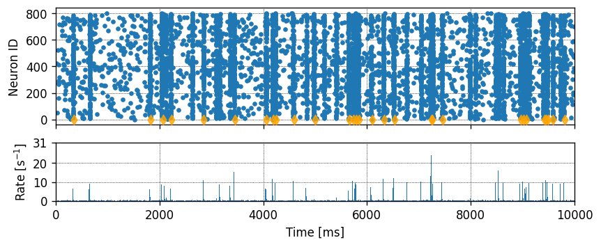
Rasterplot of network activity
N.B. orange diamonds indicate dopamine spikes.
[22]:
def _histogram(a, bins=10, bin_range=None, normed=False):
    """Calculate histogram for data.

    Parameters
    ----------
    a : list
        Data to calculate histogram for
    bins : int, optional
        Number of bins
    bin_range : TYPE, optional
        Range of bins
    normed : bool, optional
        Whether distribution should be normalized

    Raises
    ------
    ValueError
    """
    from numpy import asarray, iterable, linspace, sort, concatenate

    a = asarray(a).ravel()

    if bin_range is not None:
        mn, mx = bin_range
        if mn > mx:
            raise ValueError("max must be larger than min in range parameter")

    if not iterable(bins):
        if bin_range is None:
            bin_range = (a.min(), a.max())
        mn, mx = [mi + 0.0 for mi in bin_range]
        if mn == mx:
            mn -= 0.5
            mx += 0.5
        bins = linspace(mn, mx, bins, endpoint=False)
    else:
        if (bins[1:] - bins[:-1] < 0).any():
            raise ValueError("bins must increase monotonically")

    # best block size probably depends on processor cache size
    block = 65536
    n = sort(a[:block]).searchsorted(bins)
    for i in range(block, a.size, block):
        n += sort(a[i:i + block]).searchsorted(bins)
    n = concatenate([n, [len(a)]])
    n = n[1:] - n[:-1]

    if normed:
        db = bins[1] - bins[0]
        return 1.0 / (a.size * db) * n, bins
    else:
        return n, bins

ev = espikes.get("events")
ts, node_ids = ev["times"], ev["senders"]
hist_binwidth = 10. # [ms]

fig, ax = plt.subplots(nrows=2, gridspec_kw={"height_ratios": (2, 1)})
ax[0].plot(ts, node_ids, ".")
ax[0].scatter(t_dopa_spikes, np.zeros_like(t_dopa_spikes), marker="d", c="orange", alpha=.8, zorder=99)
ax[0].set_ylabel("Neuron ID")

t_bins = np.arange(
    np.amin(ts), np.amax(ts),
    float(hist_binwidth)
)
n, _ = _histogram(ts, bins=t_bins)
num_neurons = len(np.unique(node_ids))
heights = 1000 * n / (hist_binwidth * num_neurons)
ax[1].bar(t_bins, heights, width=hist_binwidth, color="tab:blue", edgecolor="none")
ax[1].set_yticks([
    int(x) for x in
    np.linspace(0, int(max(heights) * 1.1) + 5, 4)
])
ax[1].set_ylabel("Rate [s${}^{-1}$]")
ax[0].set_xticklabels([])
ax[-1].set_xlabel("Time [ms]")
for _ax in ax:
    _ax.set_xlim(0., total_t_sim)
plt.show()
plt.close(fig)
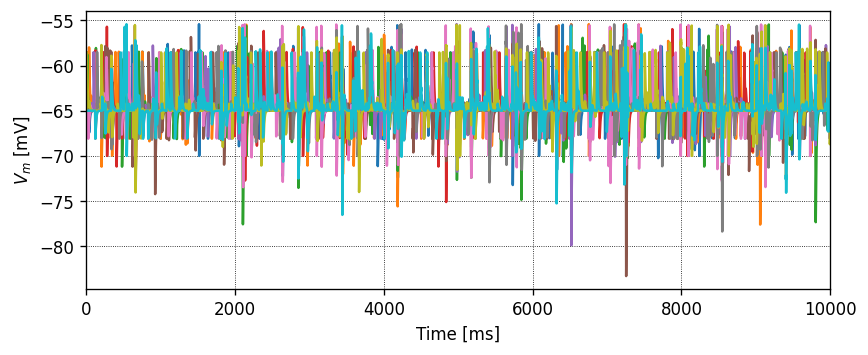
Plot membrane potential of 10 random excitatory cells
This helps to check if the network is in a balanced excitation/inhibition regime.
[23]:
fig, ax = plt.subplots()
for i in range(10):
    ax.plot(mms[i].get("events")["times"], mms[i].get("events")["V_m"], label="V_m")
ax.set_xlim(0., total_t_sim)
ax.set_ylabel("$V_m$ [mV]")
ax.set_xlabel("Time [ms]")

plt.show()
plt.close(fig)
Timeseries
We should verify that the dopamine concentration is the same in group and nongroup neurons.
Note that the timeseries resolution (due to the chunking of the simulation) could be too low to see fast dopamine dynamics. Use more chunks to increase the temporal resolution of this plot, or fewer to speed up the simulation. Consider the relationship between \(\tau_d\) and how many chunks we need to adequately visualize the dynamics.
[24]:
fig,ax = plt.subplots()

ax.plot(log["t"], log["reinforced_group"]["n_avg"], label="avg dopa group", linestyle=":", markersize=10, alpha=.7, marker="x")
ax.plot(log["t"], log["not_reinforced_group"]["n_avg"], label="avg dopa nongroup", linestyle="--", alpha=.7, marker="o")
ax.legend()

ax.set_xlim(0., total_t_sim)
ax.set_xlabel("Time [ms]")
ax.set_ylabel("Dopamine concentration [a.u.]")

plt.show()
plt.close(fig)
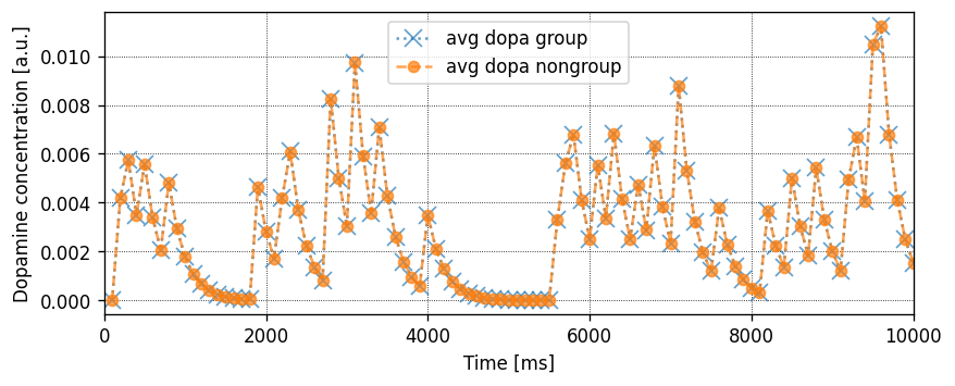
In any case, all synapses seem to be receiving the same dopamine signal.
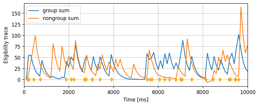
Now plot the average eligibility trace \(c\) for group and nongroup neurons:
[25]:
fig,ax = plt.subplots(figsize=(8, 3))
ax.plot(log["t"], log["reinforced_group"]["c_sum"], label="group sum")
ax.plot(log["t"], log["not_reinforced_group"]["c_sum"], label="nongroup sum")
ax.scatter(t_dopa_spikes, np.zeros_like(t_dopa_spikes), marker="d", c="orange", alpha=.8, zorder=99)
ax.set_xlim(0., total_t_sim)
ax.set_xlabel("Time [ms]")
ax.set_ylabel("Eligibility trace")
ax.legend()

plt.show()
plt.close(fig)
[26]:
fig,ax = plt.subplots(nrows=2, gridspec_kw={"height_ratios": (2, 1)})

ax[0].plot(log["t"], log["reinforced_group"]["w_avg"], label="group")
ax[0].plot(log["t"], log["not_reinforced_group"]["w_avg"], label="nongroup")
ax[0].plot(log["t"], log["w_net"], label="net")
ax[1].plot(log["t"], np.array(log["reinforced_group"]["w_avg"]) - np.array(log["not_reinforced_group"]["w_avg"]),
           label="group - nongroup", c="tab:red")
for _ax in ax:
    _ax.legend()
    _ax.set_xlim(0., total_t_sim)

ax[-1].set_xlabel("Time [ms]")
ax[0].set_xticklabels([])
ax[0].set_ylabel("Average weight                                                                     ")

plt.show()
plt.close(fig)
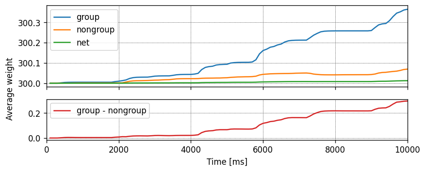
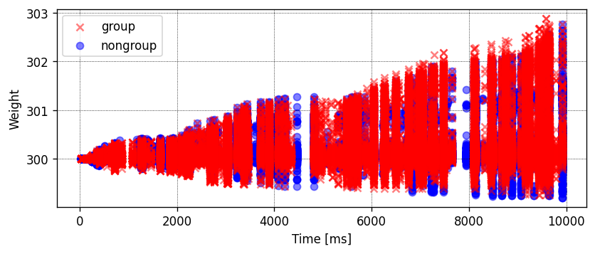
We can also plot all subgroup_size weights over time for the reinforced and non-reinforced groups as a scatterplot.
[27]:
group_weight_times = [[] for _ in range(n_subgroups)]
group_weight_values = [[] for _ in range(n_subgroups)]

senders = np.array(wr.events["senders"])

for subgroup_idx in range(n_subgroups):
    nodes_ex_gids = nodes_ex[subgroup_indices[subgroup_idx]].tolist()
    idx = [np.where(senders == nodes_ex_gids[i])[0] for i in range(subgroup_size)]
    idx = [item for sublist in idx for item in sublist]
    group_weight_times[subgroup_idx] = wr.events["times"][idx]
    group_weight_values[subgroup_idx] = wr.events["weights"][idx]

fig, ax = plt.subplots()
for subgroup_idx in range(n_subgroups):
    if subgroup_idx == reinforced_subgroup_idx:
        c = "red"
        zorder = 99
        marker = "x"
        label = "group"
    else:
        c = "blue"
        zorder=1
        marker = "o"
        label = "nongroup"

    ax.scatter(group_weight_times[subgroup_idx], group_weight_values[subgroup_idx], c=c, alpha=.5, zorder=zorder, marker=marker, label=label)

ax.set_ylabel("Weight")
ax.set_xlabel("Time [ms]")
ax.legend()

plt.show()
plt.close(fig)
Citations
[1] Mikaitis M, Pineda García G, Knight JC and Furber SB (2018) Neuromodulated Synaptic Plasticity on the SpiNNaker Neuromorphic System. Front. Neurosci. 12:105. doi: 10.3389/fnins.2018.00105
[2] PyGeNN: A Python library for GPU-enhanced neural networks, James C. Knight, Anton Komissarov, Thomas Nowotny. Frontiers
[3] Eugene M. Izhikevich. Solving the distal reward problem through linkage of STDP and dopamine signaling. Cerebral Cortex 17, no. 10 (2007): 2443-2452.
[4] Nicolas Brunel. Dynamics of sparsely connected networks of excitatory and inhibitory spiking neurons. Journal of Computational Neuroscience 8(3):183-208 (2000)
Acknowledgements
This software was developed in part or in whole in the Human Brain Project, funded from the European Union’s Horizon 2020 Framework Programme for Research and Innovation under Specific Grant Agreements No. 720270, No. 785907 and No. 945539 (Human Brain Project SGA1, SGA2 and SGA3).
The authors would like to thank James Knight, Garibaldi García and Mantas Mikaitis for their kind and helpful feedback.
License
This notebook (and associated files) is free software: you can redistribute it and/or modify it under the terms of the GNU General Public License as published by the Free Software Foundation, either version 2 of the License, or (at your option) any later version.
This notebook (and associated files) is distributed in the hope that it will be useful, but WITHOUT ANY WARRANTY; without even the implied warranty of MERCHANTABILITY or FITNESS FOR A PARTICULAR PURPOSE. See the GNU General Public License for more details.